
Effendi Tri Bahtiar
Faculty of Forestry, Bogor Agricultural University, Campus IPB Darmaga, West Java, Indonesia
Atmawi Darwis
School of Life Sciences and Technology, Bandung Institute of Technology, West Java, Indonesia
Journal of Biological Sciences
Year: 2014 | Volume: 14 | Issue: 3 | Page No.: 183-194


ABSTRACT
Sigmoid curve was well known as a general curve to fit the growth behavior of cell, organism, or population in accordance with limitation of genetic, environmental capacity and density in their habitat. Unfortunately, many growth behaviors did not follow the basic sigmoid curve because the prerequisite assumptions were not fulfilled by actual condition. In this study, linear and nonlinear function were used to modify the exponential curve become a new growth curve which could be used in more general cases than available model nowadays. Linear modification developed basic sigmoid curve. Nonlinear functions were proposed to modify the exponential curve in this study were named after: Second order polynomial (quadratic), logarithm and second order logarithm. Basic sigmoid curve and logarithm modification on exponential curve resulted curve which always had one asymptote line so it was suitable for fitting the fiber length data at every growth ring if the samples were completely made from juvenile and mature period. If the samples came from the juvenile period alone or the researcher had not certainly sure yet, quadratic or second order logarithm modification were highly recommended to be used because those equations could result two, one, or none asymptote line. Second order logarithm was generally become the best one among others. Mathematical curve fitting on fiber length growth in this study was successfully pointed the transitional age of juvenile/mature period of Teakwood with high coefficient of determination and low standard deviation. Based on recommended mathematical method, the transitional age of Teakwood was 9-12 years old. It was more precise than visual assessment conducted by 30 undergraduate students in wood science and technology class in Bogor Agricultural University which resulted 7-15 years old. The mathematical method reduced the subjectivity and variability compared to visual assessment.
PDF Abstract XML References Citation
Received: September 22, 2013;
Accepted: December 19, 2013;
Published: February 04, 2014
How to cite this article
Effendi Tri Bahtiar and Atmawi Darwis, 2014. Exponential Curve Modification by Linear and Nonlinear Function to Fit the
Fiber Length of Teakwood (Tectona grandis). Journal of Biological Sciences, 14: 183-194.
DOI: 10.3923/jbs.2014.183.194
URL: https://scialert.net/abstract/?doi=jbs.2014.183.194
DOI: 10.3923/jbs.2014.183.194
URL: https://scialert.net/abstract/?doi=jbs.2014.183.194
INTRODUCTION
Background: Mathematical knowledge is a basic science which becomes general requirement for every researcher to support their research. Mathematical procedures offer some premises in order to find the reasonable solution for many problems in scientific field such as biology and ecology. Studies on the growth of cell, organism and population are some biological aspects where the mathematical knowledge provides very important and valuable contributions. Malthusian growth curve which was drawn from exponential equation has become basic mathematical procedure to develop growth models (Pielou, 1977). Then a Belgian mathematics Pierre-Francois Verhulst (1804-1849) developed the Malthusian model become logistic equation which have an asymptote line (K) (Kucharavy and De Guio, 2007; Tsoularis and Wallace, 2002). The asymptote line showed the maximum parameter of the object (e.g., size of cell or organism, quantity of individual in a population) as a result of interaction between genetic, environmental capacity and density of cells, organisms, or population in their habitat. The Verhust-Pearl model was built by modifying the exponential curve with a linear function. The model was drawn as sigmoid (“S”) curve which have a symmetric line when the response reached a half of asymptote (K/2).
Sigmoid curve has been well known as generic solution for explaining many growth behaviors (Kucharavy and De Guio, 2007). Unfortunately, there are some growth behaviors which did not follow the basic sigmoid curve. Some cells, organisms, or population do not have the symmetric line at K/2 because of some reasons, e.g., (1) The intrinsic rate of increase in beginning (young) age was not equal to the decrease rate in final (mature and old) age; (2) The environmental capacity was not constant which presented some disturbances in environmental condition during the organism growth period; (3) The effect of density was not constant for all age. This research was conducted in order to offer more alternative mathematical solution for fitting the growth curve more precisely. Some nonlinear equations were applied to modify the Malthusian exponential model become new models. The asymptote line (K) for each model formulated when the intrinsic growth rate had zero value because there will be no growth anymore after this line. Then the model was drawn into graphical sketch in order to fit the empirical measurement.
Empirical study was conducted by measuring the fiber length growth of Teakwood (Tectona grandis) which was cut from five age tree classes. The fiber length of wood will be longer in outer growth ring because the cambial- initial length in mature age tree are longer in size than the younger one. Variation in length of xylem elements reflects the principal size changes in the cambial initials (Philipson and Butterfield, 1968). The fiber length of the young tree grows with the accelerated rate, but the intrinsic rate of increasing growth becomes slower when the tree is getting older. At a certain point the rate of increasing growth has zero value. This point is called inflection point where the growth rate decreases afterward. The fiber length becomes constant when there is no growth anymore. This condition was described by asymptote line. When the measured fiber length was longer than asymptote line value, the juvenile wood period ended and the tree was appointed as mature. Juvenile wood (sometimes called core wood) is formed near the pith and is characterized by progressive increasing of the cell dimension especially its fiber length, while the fiber length in mature wood is commonly constant.
Aim and scope: This research generally aims to develop an alternative mathematical model for fitting the growth curve which could be used in biological and ecological study. The specific aim of this research is to fit the wood fiber length of Teakwood with the linear and nonlinear modified exponential model and then appoint the transitional age which is defined as the growth ring number where the juvenile wood period ends and the tree becomes mature.
THEORETICAL BASIS
Malthus developed a discrete equation for sketching a growth curve (Eq. 1):
| (1) |
The parametric solution of Eq. 1 was obtained from integration becoming exponential equation (Eq. 2):
| (2) |
The growth curves which were drawn from Eq. 1 or 2 kept going up until unlimited threshold. This condition is irrational because growth is always limited by genetic, environmental capacity and the density of population. Interaction of the three components results the decreasing of growth rate so that at a particular point the maximum growth parameter is reached. This maximum parameter is denoted by an asymptote line (K) in growth curve. Verhulst-Pearl modifies the Malthus model with linear function which becomes Eq. 3:
| (3) |
The maximum growth parameter (K) is reached when the first derivation of growth equation has zero value (Eq. 4). K is an asymptote line:
| (4) |
| (5) |
For fitting more general cases, some nonlinear equation could be used to modify the exponential growth equation. The general term for nonlinear modification of exponential models were shown as Eq. 6:
| (6) |
Notation f(N) is a generic function which could be substituted by a constant, linear, polynomial, or logarithm equation. If f(N) is constant (f(N) = a), it is definitely equal to classic Malthus exponential model. If f(N) is linear function (f(N) = a+b(N)), the equation becomes logistic Verhulst-Pearl (sigmoid) curve. This research was conducted by substituting the f(N) function with nonlinear equation namely: Second order polynomial, logarithm and second order logarithm.
Second order polynomial (quadratic): The basic equation for quadratic modification is Eq. 7:
| (7) |
And the asymptote line (K) could be appointed by Eq. 8:
| (8) |
Logarithm: The basic equation is Eq. 9:
| (9) |
And the asymptote line (K) is:
| (10) |
Second order logarithm:
| (11) |
And the asymptote line (K) is:
| (12) |
It is possible to obtain one or two solutions for each Eq. 8 and 12. If there are two solutions, the rational and reasonable value should be chosen. The solutions for Eq. 8 and 12 sometimes are imaginary numbers. In this circumference, it could be concluded that all measured data come from young (juvenile) object because there is no asymptote line.
The reliability of a model is justified by its coefficient of determination (R2). The higher value of R2 means better reliability. In this research, R2 is calculated by Eq. 13:
 | (13) |
MATERIALS AND METHODS
Sampling method and fiber length measurement: Five Teakwood trees (Tectona grandis L.f.) on various age-classes in plantation forest which belong to Perum Perhutani BKPH Nglebur KPH Cepu were cut down with legal permission signed by Ir Sadharjo Siswamartana M.Sc., the Head of Research and Development Center PT Perhutani. The age of each tree was 9 (KU1), 12 (KU2), 25 (KU3), 35 (KU4) and 45 (KU5) years old. Then a disc was made by cutting each tree at 130 cm height. The thickness of each disc was 5 cm. The discs were sanded with fine sandpaper so that the growth rings were clearly visible. Maceration was done for each growth ring; starting from the first growth ring near the pith to the final growth ring near the cambium. A microscope which is equipped with ruler scale at the objective lens was used to measure the fiber length. The sample replications were 45 fibers for each growth ring.
Visual assessment of transitional age: The fiber length data was plotted in Cartesian diagram. Then the graph was showed to undergraduate student in wood science and technology class in Faculty of Forestry, Bogor Agricultural University. Multiple choice questions were given to 30 students. The question was: “Juvenile period of wood is defined by the progressive change in cells dimension, especially its fiber length, while the dimension of cells in mature period are relatively constant. The transitional age is the point where the juvenile period ends and the mature period begins. According to the graph for each age class shown below, when did the transitional age of wood occur?” Every student answered the question by circling their choice either in 5th, 6th, 7th, 8th, 9th, 10th, 11th, 12th, 13th, 14th, 15th, 16th, 17th, 18th, 19th, 20th growth ring or all samples come from juvenile wood. The students’ choices were described by descriptive statistics in order to measure its variability.
Mathematical assessment of transitional age: Data analysis was conducted by regression analysis:
| • | Linear: |
yi = a+bxi+εi | (14) |
| • | Second order polynomial: |
yi = axi2+bxi+c+εi | (15) |
| • | Logarithm: |
yi = aln(xi)+b+εi | (16) |
| • | Second order logarithm: |
yi = a(ln(xi))2+bln(xi)c+εi | (17) |
Where:
| (18) |
xi = Ni | (19) |
Ni = Fiber length at ith growth ring
εi = Residual at ith growth ring
The graphical solution for each growth model is sketched in Cartesian diagram based on Eq. 20 and 21:
| (20) |
| (21) |
Fiber length which estimated value at the first growth ring (![]() ) was calculated by iteration method minimizing the sum square of residual thus the coefficient of determination reached its maximum value. The asymptote line (K) calculated by Eq. 5, 8, 10 and 12 for linear, quadratic, logarithm and 2nd order logarithm model, respectively. The transitional age was appointed when the empirical measurement was higher than the asymptote line at the first time. In this research, the fiber lengths were measured for every growth ring and one growth ring represented 1 (one) year of growth, so the dt = (ti+1-ti) value in Eq. 18 and 21 is equal to 1 (one). The coefficient of determination was calculated by Eq. 13, while the pooled standard deviations (s) were measured by Eq. 22:
) was calculated by iteration method minimizing the sum square of residual thus the coefficient of determination reached its maximum value. The asymptote line (K) calculated by Eq. 5, 8, 10 and 12 for linear, quadratic, logarithm and 2nd order logarithm model, respectively. The transitional age was appointed when the empirical measurement was higher than the asymptote line at the first time. In this research, the fiber lengths were measured for every growth ring and one growth ring represented 1 (one) year of growth, so the dt = (ti+1-ti) value in Eq. 18 and 21 is equal to 1 (one). The coefficient of determination was calculated by Eq. 13, while the pooled standard deviations (s) were measured by Eq. 22:
| (22) |
where, n = No. of samples, p = No. of parameters (3 for linear and logarithm modification and 4 for quadratic and second order polynomial modification).
RESULTS
Visual assessment of transitional age: The measurements of Teakwood fiber length in correlation with growth ring number from the pith were shown in Fig. 1. As seen on Fig. 1 the fiber length were progressively changing in the beginning, then relatively constant in the end. The period when the progressive change occurred is defined as juvenile wood period; while the constant period is defined as mature. The visual assessment could be done to justify the transitional age where the juvenile period ended and the mature period began, but it is very subjective depending on the observer’s view. The author showed the graphs as seen on Fig. 1 and asked 30 undergraduate students in wood science and technology class in Faculty of Forestry-Bogor Agricultural University to point a coordinate where the transitional age occurred by visual assessment. The questions were in multiple choices type. Each student gave various answers as seen on Fig. 2. The variation value was high enough. The students’ answers range for KU1 was 7th-9th but some students chose they were all juvenile while for KU2 was 7th-12th and some also answered all juvenile. KU3 was 12th-15th, KU4 was 9th-13th and KU5 was 11th-13th. Most of students chose the 8th, 9th, 12th, 13th and 11th growth ring as the transitional age of Teakwood at KU1, KU2, KU3, KU4 and KU5 age class, respectively. In order to reduce the variability and subjectivity in pointing the transitional age, mathematical method should be developed.
Mathematical assessment of transitional age: Mathematical method which was proposed to fit the fiber length growth of Teakwood in this research is general exponential curve which was modified by linear and nonlinear function. Linear function modified the exponential curve becoming sigmoid curve. Second order polynomial, logarithm and second order logarithm function were chosen to modify the basic exponential curve becoming a new growth curve.
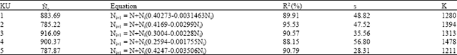
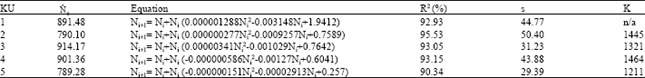
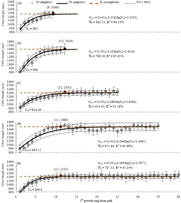
Sigmoid curve: The sigmoid curve equation which fit the fiber length of Teakwood at every growth ring was shown in Table 1 and the graph was shown in Fig. 3.
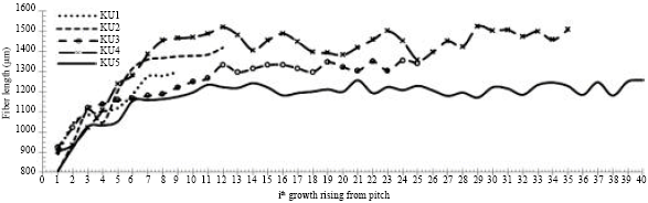 | |
| Fig. 1: | Fiber length of Teakwood in every growth ring for five tree age classes |
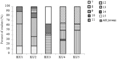 | |
| Fig. 2: | Undergraduate student’s visual assessment to point the transitional age of Teakwood (n = 30 students) |
| Table 1: | Equation and asymptote of sigmoid curve for fitting the fiber length of Teakwood |
 | |
| KU = Age class; | |
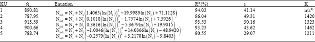
| Table 2: | Equation and asymptote of exponential curve modification by quadratic function for fitting the fiber length of Teakwood |
 | |
| KU = Age class; | |
The coefficients of determination (R2) values were high for each equation (88-96%) and the standard deviations were small enough compared to the average fiber length. This condition proved that sigmoid curve was good enough to fit the fiber length of Teakwood at every growth ring. The sigmoid curve had asymptote line (K) that is a horizontal threshold where the function result was almost a constant value. This constant value will be reached by the function when Ni is infinite.
As seen on Fig. 3, the average Teakwood fiber length measurements were higher than asymptote line at the first time at 9th, 12th, 12th, 11th and 11th growth ring for KU1, KU2, KU3, KU4 and KU5, respectively. It means the juvenile period ended at those growth rings and the mature period began. This point was called transitional age of wood. It was confident enough that the transitional age of KU3, KU4 and KU5 was on the 12th, 11th and 11th growth ring respectively, but it was doubtful for KU1 and KU2 because only one data value was higher than the asymptote and the point was at the butt end of graph. In this case, the author preferred to decide that all KU1 and KU2 samples came from juvenile wood. The linear modification could give a good and reasonable function if the data certainly came from the juvenile and mature period of wood. If all samples were made from juvenile period, or the researcher was not so certain, it is not recommended to use sigmoid curve to fit the fiber length growth and justify the transitional age of wood.
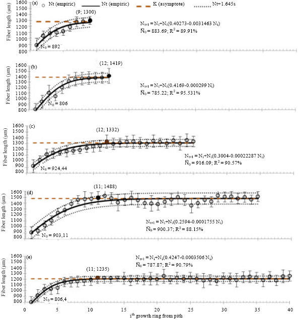
Second order polynomial modification: Second order polynomial (quadratic) function modification could give more reasonable result to fit the fiber length of wood than the sigmoid curve because it could have two, one, or none of asymptote depend on the data. If all data came from juvenile wood, there would not have been any asymptote. The equation of quadratic modification and its asymptote were tabulated in Table 2, while the graphs were in Fig. 4. The models gave high reliability because the coefficient of determination (R2) of each equation was high and the pooled standard deviation (s) was small enough.
There were 4 parameters in quadratic modification namely: An intercept (c), two regression coefficients (a and b) and an estimated fiber length at the first growth ring (![]() ).
).
 | |
| Fig. 3(a-e): | Sigmoid curve fitting for fiber length growth of (a) KU1, 9, (b) KU2, 12, (c) KU 3, 25, (d) KU4, 35 and (e) KU 5, 45 years old teakwood |
Quadratic modification used only one additional parameter compared to linear modification. If the researcher was not certain that the data came from juvenile and mature period of wood, the additional parameter should play significant role in curve fitting.
Since the solutions for quadratic equation for KU1 were imaginary numbers, there was not any asymptote line drawn. This condition proved that all samples from KU1 were juvenile wood; there was not a mature part of the wood. For KU2, the rational asymptote line was 1445 μm but there had not been any fiber length measurement reached that value yet. All of the data were below the asymptote line. So it could be concluded that the Teakwood from KU2 was still in juvenile period. While mature period of KU3, KU4 and KU5 began at 12th, 9th and 11th, respectively, because the fiber length measurements at those points were higher than the asymptote line at the first time (Fig. 4).
Logarithm modification: Similar with linear modification, a logarithm modification for exponential curve always results a curve with an asymptote line. So it was suitable to fit the fiber length if the data consisted of juvenile and mature period of wood. It is not recommended if the data come from the juvenile part of wood only.
 | |
| Fig. 4(a-e): | Quadratic modification of exponential curve fitting for fiber length growth of (a) KU1, 9, (b) KU2, 12, (c) KU3, 25, (d) KU4, 35 and (e) KU5, 45 years old teakwood |
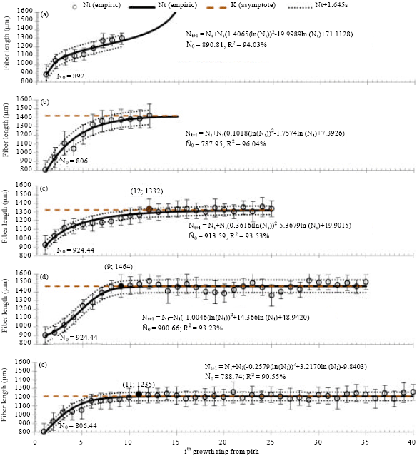
| Table 3: | Equation and asymptote of exponential curve modification by logarithm function for fitting the fiber length growth of Teakwood |
 | |
| KU = age class; | |
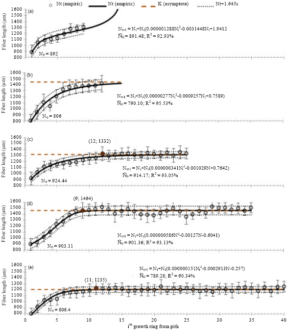
The equations of logarithm modification for exponential curve were shown in Table 3 and the graphs were in Fig. 5.
 | |
| Fig. 5(a-e): | Logarithm modification of exponential curve fitting for fiber length growth of (a) KU1, 9, (b) KU2, 12, (c) KU3, 25, (d) KU4, 35 and (e) KU5, 45 years old teakwood |
Both logarithm modification and linear modification had three parameters namely an intercept, a regression coefficient and an estimated fiber length at the first growth ring. The reliability of logarithm modification for fitting the fiber length of Teakwood at every growth ring was commonly better than linear modification because it had higher coefficient of determination (R2) and lower standard deviation (s). As seen on the graphs in Fig. 5, the fiber length measurement were higher at the first time at 9th, 12th, 12th, 11th and 11th growth rings for KU1, KU2, KU3, KU4 and KU5, respectively. Both linear and logarithm modification resulted the same transitional age values.
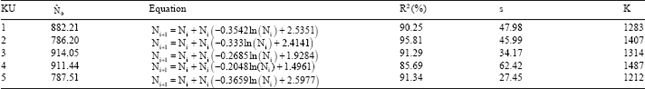
Second order logarithm modification: Second order logarithm modification gave the best result for fitting the fiber length of Teakwood at every growth ring among others. It had similar properties with quadratic modification; two, one, or none of asymptote could be found depend on the data. Both quadratic and second order logarithm modification were suitable for fitting fiber length of Teakwood whether the samples came from the juvenile only or the juvenile and mature portion of the wood. Second order logarithm modification had higher coefficient of determination and lower standard deviation compared to quadratic modification.
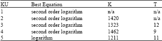
| Table 4: | Equation and asymptote of exponential curve modification by second order logarithm function for fitting the fiber length growth of Teakwood |
 | |
| KU: Age class, | |
 | |
| Fig. 6: | Second order logarithm modification of exponential curve fitting for fiber length growth of (a) KU1, 9, (b) KU2, 12, (c) KU3, 25, (d) KU4, 35 and (e) KU5, 45 years old teakwood |
As seen on Table 4, the coefficient of determination (R2) for each equation was higher than 90% and the standard deviation (s) was below 50. There was not any asymptote found for KU1 because the progressive change still occurred. It could be concluded that all samples from KU1 Teakwood were juvenile wood.
The plots of estimated result of second order logarithm modification and empirical measurement were shown in the graph in Fig. 6. As seen on Fig. 6, none of fiber length measurements of KU2 Teakwood reached its asymptote. Since, all of the measurement values were below the asymptote line, KU2 Teakwood was still in juvenile period. The fiber length measurement of KU3, KU4 and KU5 were higher than the asymptote line at the first time when the growth ring numbers were 12, 9 and 11, respectively. So, the transitional age of KU3, KU4 and KU5 were 12, 9 and 11 years old, respectively.
DISCUSSION
Juvenile wood was formed in the beginning phase of tree growth. Juvenile wood was secondary xylem which was made from young vascular cambium when apical meristem activity was significantly affected to cambium activity because they have not been in the long distance yet. It was not the growth rate which affected juvenile period but the age of the tree. Cameron et al. (2005) reported that there is a more or less fixed period of juvenile wood formation that appears to be under strong genetic control. The length of tree’s juvenile period varied between species; it was commonly before the 5th-20th growth ring from the pith (Bowyer et al., 2003). Wood which was formed in the beginning phase of the tree growth was commonly characterized by lower density, shorter fiber length and higher micro fibril angle. The properties were progressively changing on the next several growth rings and then they were slowly similar to mature wood which had relatively constant properties.
The fiber length measurement at every growth ring was proposed as a method to identify the transitional age of juvenile to mature period of wood. The age of cambium when growth rings were formed had the major effect on the variability of anatomical characteristics of wood (Bailey, 1920). The older cambium cells were longer in size than the younger ones. The initial cambial-length directly related to the fiber length of wood, thus the fiber length gradually changed in the stem, ring by ring-from the pith outward until near the cambium. At juvenile period the fiber length were changing progressively and became constant in the mature period. The transitional age could be justified as the point where the fiber length began to be constant. This point could be identified by visual assessment on the graph of fiber length versus its growth ring number, but it raised subjective and high variability results.
Visual assessment relied on human eye’s capability for distinguishing an object. The optical apparatus in human eye in association with central nervous system circuitry caused a high resolving power. Judd (1952) reported that the human eye is able to discriminate at least 10 million different colors, shades and hues. Daniels Jr. and Imbrie (1958) reported that there are some factors which produce some error in visual valuation namely the spectral color of the viewing light, color of the surrounding objects and background and colors previously seen. These errors could be corrected by brain which had been well trained daily in interpreting the effect of light, background and expectation.
Visual assessment had become well known method in many fields of study e.g., radiography, wood strength grading, historical building evaluation, etc. For reducing its subjectivity and upgrading its accuracy some scientists developed some numerical methods to equip the visual assessment. Bath and Mansson (2007) developed Visual Grading Characteristic (VGC) analysis as a non-parametric rank-invariant statistical method for evaluation the image quality of radiograph. Wu et al. (2006) invented semi-quantitative analysis to improve the visual grading system accuracy for invasive cervical carcinoma prognostic. Firmanti et al. (2005) developed a mechanical stress grading for tropical wood which improve the timber visual grading accuracy. Piazza and Riggio (2008) reported that visual grading alone result less precise information about element behavior in old timber structure; the obtained data should be critically analyzed in order to estimate the mechanical properties of member and set up reliable engineering numerical models for structural analysis.
Similar with other visual assessment in many fields, transitional age determination of wood by visual assessment produced high variability result. Each observer pointed a different growth ring at a fiber length curve of teakwood which considered as the transitional age. There is no universally accepted point of transitional age of juvenile/mature wood. In this study, students pointed the transitional age of KU1 Teakwood was 7th-9th and all juvenile, KU2 was 7th-12th and all juvenile, KU3 was 12th-15th, KU4 was 9th-13th and KU5 was 11th-13th. So based on the visual assessment, the transitional age of Teakwood was 7th-15th years old. This range was long enough because of observer’s subjectivity which produced high variability.
The mathematical method could reduce the variability so every observer would consider the same estimated transitional age of wood juvenile/mature period for each tree. This study proposed four mathematical equations which could be considered as standard function for estimating the transitional age of wood juvenile/mature period by fitting its fiber length at each growth ring,namely logistic (sigmoid) curve, quadratic modification, logarithm modification and second order logarithm modification for exponential curve. Each equation had similar characteristic with fiber length growth which was progressively changing in the beginning (juvenile) period and relatively constant at mature age period.
Sigmoid curve and logarithm modification on exponential curve always caused an asymptote line, so it was suitable for fitting the fiber length in long period of tree growth which consisted of juvenile and mature period.
| Table 5: | Best equation modification of exponential curve for fitting the fiber length growth of Teakwood and its transitional age point |
 | |
| K = asymptote and T = transitional age | |
If the data came from the juvenile period alone, or the researcher had not been certain yet, the quadratic or second order logarithm modification on exponential curve were highly recommended to be used because these types of curve could have two, one, or none asymptote line depending on the data. If the data came from juvenile period alone, there would not be any asymptote line in quadratic and second order modification of exponential curve because the mathematic solutions were imaginary number.
Logarithm modification on exponential curve was better than logistic (sigmoid) curve in fitting the fiber length growth. Second order logarithm generally became the best among others because it had highest coefficient of determination (R2) and lowest standard deviation (s). The best equation for each age class of Teakwood was shown in Table 5. As seen on Table 5, it was confident enough to conclude that Teakwood was in transitional age period at 9-12 years old based on mathematical equation. At that age, the juvenile period ended and the mature period began.
CONCLUSION
Basic sigmoid curve and logarithm function modification on exponential was suitable for fitting the fiber length data at every growth ring if the samples were completely made from juvenile and mature period of wood. If the samples came from the juvenile period alone or the researcher had not been certain yet, quadratic and second order logarithm modification on exponential curve was highly recommended. Logarithm equation was better than linear, while second order logarithm was better than quadratic. Second order logarithm had generally become the best one among others. Mathematical curve fitting on fiber length growth in this study had successfully pointed the transitional age of juvenile/mature period of Teakwood with high coefficient of determination and low standard deviation. Based on recommended mathematical method, the transitional age of Teakwood was 9-12 years old. It was more precise than visual assessment conducted by 30 (thirty) undergraduate students in wood science and technology class in Faculty of Forestry-Bogor Agricultural University which resulted 7-15 years old. The mathematical method reduced the subjectivity and variability compared to visual assessment.
ACKNOWLEDGEMENT
The authors thank to Ir Sadharjo Siswamartana MSc, The Head of R and D PT Perhutani for his beneficial contribution so this research could be conducted in PT Perhutani, BKPH Nglebur KPH Cepu. Thanks are also due to the Directorate General of Higher Education-Indonesian Ministry of Education on the permit so that the authors have the time and opportunity to do this research.
REFERENCES
- Bath, M. and L.G. Mansson, 2007. Visual grading characteristics (VGC) analysis: A non-parametric rank-invariant statistical method for image quality evaluation. Br. J. Radiol., 80: 169-176.
CrossRefPubMedDirect Link - Cameron, A.D., S.L. Lee, A.K. Livingston and J.A. Petty, 2005. Influence of selective breeding on the development of juvenile wood in Sitka spruce. Can. J. For. Res., 35: 2951-2960.
CrossRefDirect Link - Daniels Jr., F. and J.D. Imbrie, 1958. Comparison between visual grading and reflectance measurements of Erythema produced by sunlight. J. Invest. Dermatol., 30: 295-304.
CrossRefDirect Link - Firmanti, A., E.T. Bahtiar, S. Surjokusumo, K. Komatsu and S. Kawai, 2005. Mechanical stress grading of tropical timbers without regard to species. J. Wood Sci., 51: 339-347.
CrossRefDirect Link - Piazza, M. and M. Riggio, 2008. Visual strength-grading and NDT of timber in traditional structures. J. Build. Appraisal, 3: 267-296.
CrossRefDirect Link - Tsoularis, A. and J. Wallace, 2002. Analysis of logistic growth models. Math. Biosci., 179: 21-55.
CrossRefPubMedDirect Link - Wu, Y.C., H.J. Yang, C.C. Yuan and K.C. Chao, 2006. Visual grading system, blood flow index and tumor marker SCC antigen as prognostic factors in invasive cervical carcinoma. J. Med. Ultrasound, 14: 25-31.
CrossRefDirect Link