Analysis of Bifurcation Phenomena of Voltage-fed inductively Coupled Power Transfer System Varying with Coupling Coefficient

This study investigates the frequency bifurcation phenomena of a typical voltage-fed resonant converter based on mutual induction model. It is found that the Zero Current Switching (ZCS) operating frequency has the bifurcation region as the coupling coefficient varies due to the distance. The expression for the bifurcation boundary is derived and analyzed. Such results are very useful for guiding the design of practical Inductively Coupled Power Transfer (ICPT) systems especially in applications which have the requirement of the position flexibility. Analytical results are verified both via MATLAB simulations and experimental prototype.

INTRODUCTION

Inductively Coupled Power Transfer (ICPT) technology allows electrical energy to be transferred from a stationary primary source to one or more movable secondary loads over relatively large air gaps (Si et al., 2008). It is widely used in special fields, such as inflammable and explosive areas and wet or undersea environment (Li et al., 2013; Wu et al., 2011). Moreover, household electric appliances, battery charging and other portable electronic devices are also beginning to apply it (Sun et al., 2012; Moradewicz and Kazmierkowski, 2010; Tian et al., 2012; Boys et al., 2007; Keeling et al., 2010).

It is well known that one of the major constraints of ICPT systems is the frequency stability, particularly at soft-switching mode which can largely reduce the loss and Electromagnetic Interference (EMI) (Hu et al., 2000). Presently, several thesis have studied the frequency bifurcation phenomena (Tang et al., 2009, 2011; Si et al., 2008). It has been pointed out that the zero phase frequency must be equal to the secondary resonant frequency so that the maximum output power could be achieved (Wang et al., 2004). Moreover, it has also been pointed out (Li et al., 2012) that, once the frequency exceeds a certain range, ICPT systems will have multiple operating conditions and system stability will be affected. So, it is crucial to maintain the frequency stability (Boys, 2000).

Obviously, the common method of maintaining the frequency stability is to ensure the reactive elements of the primary part and secondary part to be suitably tuned (Sun et al., 2005). Although the ICPT system is completely tuned, frequency bifurcation phenomena are still caused by parameter variations, particularly small changes in load (Wang et al., 2004). Current studies which assuming the coupling coefficient to be constant mainly focus on the bifurcation caused by load variation. The stable operation boundary condition of the system has been given (Wu et al., 2004; Wei and Houjun, 2007), which consists of the secondary quality factor and the coupling coefficient.

However, for the ICPT system, in many applications especially household appliances in kitchen, the coupling coefficient which is determined by the geometrical structure and performance parameters of the magnetic structure is not always to be constant. It will change as the distance between the primary and secondary side varies (Kurschner et al., 2011).

Few researches have been done on the frequency stability with the coupling coefficient variation. It is pointed out that the efficient of the magnetically coupled resonator changes as the coupling coefficient varies and the frequency splitting phenomena occur (Sample et al., 2011), however, it does not give the expression for the bifurcation boundary.

This study uses the typical voltage-fed ICPT system as an example. An equivalent circuit model based on mutual induction model has been presented to investigate the frequency bifurcation phenomena. The frequency stability with the coupling coefficient variation has been discussed in detail and the expression for the bifurcation boundary is derived. Simulations and experiments have been carried out to verify the theoretical results.

VOLTAGE-FED ICPT SYSTEM TOPOLOGY

The ICPT system can be classified by voltage-fed system and current-fed system.

Fig. 1:

Typical voltage-fed ICPT system, Ein: DC input supply, S1-S4: Metal-oxide-semiconductor field-effect transistor (MOSFETs), Cp: Primary resonant capacitance, Rp: Resistance of primary inductor, Lp: Primary resonant inductance, iLp: Current of the primary inductor, M: Mutual inductance, Ls: Secondary resonant inductance, Rs: Resistance of secondary inductor, Cs: Secondary resonant capacitance, iLs: Current of the secondary inductor, RL: Resistance of the load, UL: Output voltage

The voltage-fed system normally matches series tuned types of resonant tanks, while current-fed system matches parallel tuned types of resonant tanks. This study investigates the frequency bifurcation phenomena of a typical voltage-fed resonant converter with the variety of the coupling coefficient. The main topology of voltage-fed ICPT system can be shown in Fig. 1.

In voltage-fed ICPT system, the high-frequency inverter comprises four MOSFET switches from S₁ to S₄. Two switch pairs (S₁, S₄) and (S₂, S₃) operate in complementary mode to invert the input DC voltage source E_in to square wave voltage output. Hence, the series network consisting of a capacitor C_p in series with an inductor L_p and a series inherent resistor R_p will produce a high-frequency sinusoidal current with low distortion. Such current provide the ZCS conditions for MOSFET switches.

In the secondary part, the pick up coil L_s receives the high-frequency energy by the magnetic fields coupling. The inductor L_s is completely tuned by the series capacitor C_s. Such resonant network converts high-frequency AC voltage supply U_L for load R_L. Resistors R_s is inherent resistance of the secondary inductor L_s. M is the mutual inductance between L_p and L_s.

BIFURCATION

The equivalent circuit of the coupling topology based on the mutual induction model is shown in Fig. 2.

Fig. 2(a-b):	Equivalent coupling circuit, Vi: Output voltage of inverter, Zi: The total impedance of the primary part, Zr: The reflected impedance, Zs: The impedance of the secondary

The impedance of the secondary is calculated as a lumped impedance whose value depends on the secondary compensation as given by:

(1)

The reflected impedance Z_r which is dependent on the transformer coupling and operating frequency is given by:

(2)

The total impedance of the primary part is:

(3)

Substituting Eq. 1 and 2 into Eq. 3, the impedance seen by the power supply can be given as:

(4)

where, the operators “Re” and “Im” represent the real and imaginary components of the input impedance:

(5)

And:

(6)

As the aim of designing the ICPT system is to deliver the power to the load, the resonant frequency of the secondary part should be chosen as the operating frequency of the system. The operating angular frequency ω₀ of the system is given by:

(7)

where, the resonant angular frequency ω₀ is defined as ω₀ = 2π f₀ and the f₀ is the operating frequency of the resonant circuit.

In addition, in order to analyze the bifurcation phenomena, the expression of the coupling coefficient k is given by:

(8)

where, the M is the mutual inductance between primary coil and secondary coil.

Here, the operating frequency (ω) is normalized using (ω₀) from Eq. 7 as:

(9)

When the whole resonant network is completely tuned, the primary impedance should satisfy:

(10)

Substituting Eq. 6-9 into Eq. 10, the imaginary components of the primary impedance is derived as:

(11)

Normally, if Eq. 11 has only one root (γ = 1), the system has only one zero phase angle resonant frequency. Apart from γ = 1, the Eq. 11 has the other sub-equation which is given as:

(12)

And the discriminant of Eq.12 is given by:

(13)

As is known, the ideal root of the Eq. 11 is γ = 1, to ensure the secondary resonant frequency is the only zero phase angle frequency, the Eq.12 must have no root (Δ<0) or the roots are invalid (Δ>0).

Fig. 3:	Relationship between Γ and the load RL

At first, letting the discriminant be zero and the coupling coefficient is given as:

(14)

Then, the Γ is define as shown below and the relationship between Γ and the load R_L is shown in Fig. 3.

(15)

Finally, the bifurcate on boundary of the coupling coefficient k are discussed in three circumstances:

•	It can be seen in Fig. 3 that when the load RL satisfy then Γ∈ (0, 1), in order to ensure the discriminant less than zero (Δ<0), the coupling coefficient k should be
•	Similarly, when the load RL satisfy then Γ∈(0, 1], in order to ensure the discriminant less than zero (Δ<0), the coupling coefficient k should be . However, the roots are invalid (Δ≥0) when the coupling coefficient k satisfy . Therefore, the coupling coefficient should be k∈ [0, 1]
•	When the load RL satisfy RL≥ (2ω0Ls-Rs) then Γ∈ (-∞, 0), all the roots are invalid (Δ≥0), thus the coupling coefficient should be k∈[0, 1]

In a word, to ensure the secondary resonant frequency is the only zero phase angle frequency, the boundary of the coupling coefficient k is given as:

(16)

The frequency bifurcation region is:

(17)

NUMERICAL VERIFICATION

In order to validate the bifurcation boundary of the system with the changes of the coupling coefficient, numerical verification with MATLAB has been carried out.

On the basis of the theory analysis discussed above, it can easily be realized the bifurcation boundary according to the parameter shown in Table 1.

It can be seen from Fig. 4a that the imaginary of the primary impedance has more than one zero-crossing point with increasing the coupling coefficient (k) at the load R_L1 = 2Ω, whereas the Fig. 4b shows that the imaginary of the primary impedance has only one zero-crossing point over a range of the coupling coefficient (k) from 0 to 1 at the load R_L2 = 12Ω. The key parameters can be calculated as and Γ = 0.076:

•	According to Eq. 16, the bifurcation boundary of the coupling coefficient k can be calculated as 0≤k≤0.2758 at the load RL1 = 2Ω
•	According to Eq. 17, the bifurcation boundary of the coupling coefficient k can be calculated 0≤k≤1 at the load RL2 = 12Ω

On the basis of the conclusion discussed above, the imaginary of the primary impedance with different coupling coefficient is shown in Fig. 5 in the form of a two-dimensional graphic representation.

Fig. 4(a-b):	Imaginary 3-D plot primary impedance with different coupling coefficient k (a) RL1 = 2Ω and (b) RL2 = 12Ω

Fig. 5(a-b):	Imaginary sketch of the primary impedance for different k (a) RL1 = 2Ω, fmin: Lower zero phase angle resonant frequency, f0: Nominal zero phase angle resonant frequency, fmax: Higher zero phase angle resonant frequency, kc: Critical coupling coefficient and (b) RL2 = 12Ω

It can be seen from Fig. 5a that there is only one operating frequency f₀ which is the ideal operating point of the system when the coupling coefficient k is >0.2758. Once the k is slightly larger than the critical value k_c (k_c = 0.2758) there are three zero phase angle resonant frequencies f_min, f₀, f_max in the primary resonant network, where f_min<f₀<f_max. Fig. 5b shows that there is only one operating frequency f₀ (f₀ = 20 kHz) at the load R_L2 = 12Ω (R_L2>10.665Ω) with the varying coupling coefficient (k).

EXPERIMENTAL RESULTS

To verify the bifurcation phenomena of ICPT system varying with coupling coefficient, a voltage-fed ICPT system shown in Fig. 1 has been implemented in a laboratory scale. The inverter consists of four MOSFETs (International Rectifier IRFB4310).The zero-crossing points of primary inductance current are detected by the current sense transformers (Talema AS-103). Phase-locked loop (CD4046) is selected to achieve the ZCS operation for the primary converter with variable frequency. The parameters of the circuit are as shown in Table 1. And the experimental results of the frequency of the voltage-fed ICPT system are shown below.

The experimental waveforms show that the system operate at ZCS condition for the input inverter voltage v_i is in phase with i_Lp, which proves that the these frequency are the zero phase frequency of the primary part of the system.

As discussed earlier, the bifurcation boundary of the coupling coefficient is 0≤k≤0.2758 at the load R_L1 = 2Ω. It can be seen from Fig. 6a that there exactly is the only one zero phase frequency f₀ (f₀ = 19.8 kHz) at the coupling coefficient k = 0.2; as the coefficient k varies from 0.1-0.4, it can be seen in Fig. 6b-d that there are three zero phase frequency of the primary current (17.8, 19.8 and 24.4 kHz, respectively).

Table 1:	Parameters of ICPT system

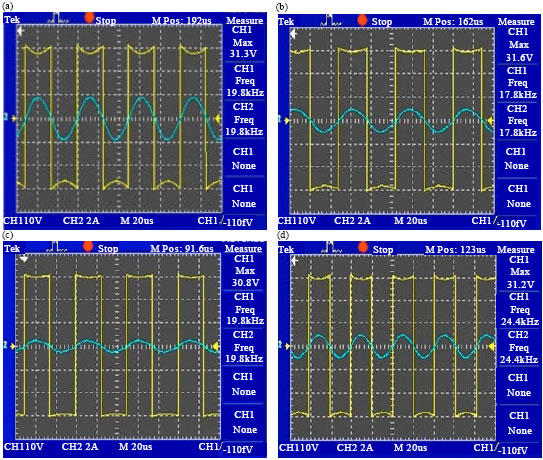Fig. 6(a-d):	Steady-state waveforms of voltage-fed ICPT system for RL1 = 2Ω (CH1: Output voltage of inverter Vi-10V/div; CH2: Current of the primary inductor iLp-2A/div) (a) f0 = 19.8 kHz, k = 0.2, (b) fmin = 17.8 kHz, k = 0.4, (c) f0 = 19.8 kHz, k = 0.4 and (d) fmax = 24.4 kHz, k = 0.4

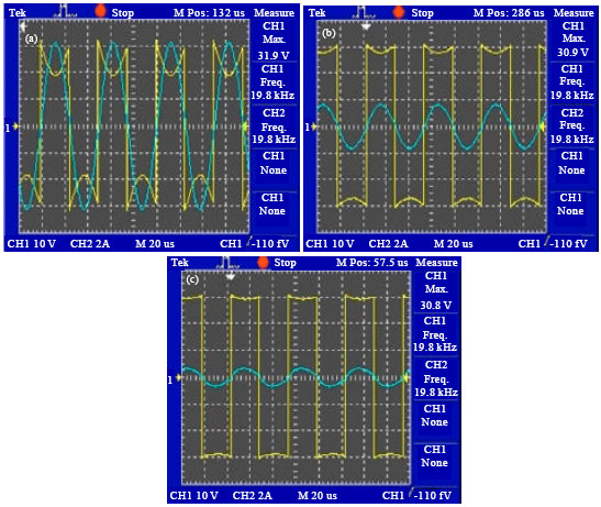Fig. 7(a-c):	Steady-state waveforms of voltage-fed ICPT system for RL2 = 12Ω (CH1: Output voltage of inverter Vi -10V/div; CH2: Current of the primary inductor iLp-2A/div) (a) f0 = 19.8 kHz, k = 0.2, (b) f0 = 19.8 kHz, k = 0.5 and (c) f0 = 19.8 kHz, k = 0.8

Fig. 8(a-b):	Practical results of the frequency of the voltage-fed ICPT system varying with coupling coefficient and ideal theoretical results (a) RL1 = 2Ω and (b) RL2 = 12Ω

However, at the light load (R_L2 = 12Ω) as shown in Fig. 7a-c, there is also exactly the only one zero phase frequency f₀ (f₀ = 19.8 kHz) over a range of coefficient k from 0.2-0.8.

As a comparison, a theoretical curve based on ideal component parameters is also plotted in Fig. 8a-b.

As shown in Fig. 8, the measured results are in good agreement with the theoretical curves. It also can be seen that the experimental curve deviates by about 0.2 kHz from the theoretical value. This is caused by deviations in actual component values from the nominal values. The theoretical results are based on the simplifications in the model that assumes sinusoidal voltages and currents and ignores losses in the capacitors and electromagnetic structure. Therefore, this error in practice doesn’t effect the analyzed results above this section.

CONCLUSION

Aimed at the frequency stability of the voltage-fed ICPT system with the coupling coefficient variation into consideration, the expression of the frequency bifurcation boundary has been analyzed and given based on mutual induction model. It is found that the bifurcation region of the zero phase resonant frequency is determined by the value range of the coupling coefficient if the load satisfies certain condition. Once the coupling coefficient exceeds a certain range, the system will have more than one zero phase frequency and the stability of the system will be affected a lot. Simulations and experiments have been carried out to validate the theoretical results and it could be useful for guiding the design of the ICPT system especially in applications which have the requirement of the position flexibility.

ACKNOWLEDGMENTS

This study is financially supported by National Natural Science Foundation of China (No.51277192, No.51207173) and Fundamental Research Funds for the Central Universities (No. CDJXS10170001). I also would like to give my special thanks to the anonymous reviewers for their contributions to this study.

REFERENCES

- Boys, J.T., G.A. Covic and A.W. Green, 2000. Stability and control of inductively coupled power transfer systems. Electric Power Appl., 147: 37-37.
CrossRef - Boys, J.T., G.A.J. Elliott and G.A. Covic, 2007. An appropriate magnetic coupling co-efficient for the design and comparison of ICPT pickups. IEEE Trans. Power Electron., 22: 333-335.
CrossRef - Hu, A.P., J.T. Boys and G.A. Covic, 2000. Frequency analysis and computation of a current-fed resonant converter for ICPT power supplies. Proceedings of the International Conference on Power System Technology, December 2000, Department of Electrical and Electronic Engineering Auckland University, Australia pp: 327-332.
CrossRef - Keeling, N.A., G.A. Covic and J.T. Boys, 2010. A unity-power-factor IPT pickup for high-power applications. IEEE Trans. Ind. Electron., 57: 744-751.
CrossRef - Kurschner, D., C. Rathge and U. Jumar, 2011. Design methodology for high efficient inductive power transfer systems with high coil positioning flexibility. IEEE Trans. Ind. Electron., 60: 372-381.
CrossRef - Li, Y.L., Y. Sun and X. Dai, 2012. Controller design for an uncertain contactless power transfer system. Inform. Technol. J., 11: 971-979.
CrossRef - Li, Y.L., Y. Sun and X. Dai, 2013. μ-Synthesis for frequency uncertainty of the ICPT system. IEEE Trans. Ind. Electron., 60: 291-300.
CrossRef - Moradewicz, A.J. and M.P. Kazmierkowski, 2010. Contactless energy transfer system with FPGA-controlled resonant converter. IEEE Trans. Ind. Electron., 57: 3181-3190.
CrossRef - Sample, A.P., D.A. Meyer and J.R. Smith, 2011. Analysis, experimental results and range adaptation of magnetically coupled resonators for wireless power transfer. IEEE Trans. Ind. Electron., 58: 544-554.
CrossRef - Si, P., A.P. Hu, S. Malpas and D. Budgett, 2008. A frequency control method for regulating wireless power to implantable devices. IEEE Trans. Biomed. Circuits Syst., 2: 22-29.
CrossRefDirect Link - Sun, Y., X. Lv, Z. Wang and C. Tang, 2012. A quasi sliding mode output control for inductively coupled power transfer system. Inform. Technol. J., 11: 1744-1750.
CrossRefDirect Link - Tang, C.S., X. Dai, Z. Wang, Y. Sun and A.P. Hu, 2011. Frequency bifurcation phenomenon study of a soft switched push-pull contactless power transfer system. Proceedings of the 6th IEEE Conference on Industrial Electronics and Applications, 21-23 June 2011, Beijing, pp: 1981-1986.
CrossRef - Tang, C.S., Y. Sun, Y.G. Su, S.K. Nguang and A.P. Hu, 2009. Determining multiple Steady-state ZCS operating points of a Switch-mode contactless power transfer system. IEEE Trans. Power Electron., 24: 416-425.
CrossRef - Tian, Y., Y. Sun, Y. Su, Z. Wang and C. Tang, 2012. Neural network-based constant current control of dynamic wireless power supply system for electric vehicles. Inform. Technol. J., 11: 876-883.
CrossRefDirect Link - Wang, C.S., G.A. Covic and O.H. Stielau, 2004. Power transfer capability and bifurcation phenomena of loosely coupled inductive power transfer systems. IEEE Trans. Ind. Electron., 51: 148-157.
CrossRef - Wei, L. and T. Houjun, 2007. Analysis of voltage source inductive coupled power transfer systems based on zero phase angle resonant control method. Proceedings of the 2nd IEEE Conference on Industrial Electronics and Applications, May 23-25, 2007, Harbin, pp: 1873-1877.
CrossRef - Wu, H.H., G.A. Covic, J.T. Boys and D.J. Robertson, 2011. A series-tuned inductive-power-transfer pickup with a controllable AC-voltage output. IEEE Trans. Power Electron., 26: 98-109.