
Chao Li
Institute of Mathematics and Statistics, Yunnan University, 2 Cuifu Northern Road, 650091, Kunming, Republic of China
Yue Zhao
Institute of Mathematics and Statistics, Yunnan University, 2 Cuifu Northern Road, 650091, Kunming, Republic of China
Information Technology Journal
Year: 2012 | Volume: 11 | Issue: 9 | Page No.: 1202-1210


ABSTRACT
Estimation of camera relative positions is very important in computer vision. Assuming that the camera has been calibrated, this study presents two algorithms of camera relative pose estimation which one is to recover the camera motion parameters by essential matrix and the other by epipolar geometry. Algorithm 1 is commonly used in three-dimensional (3D) reconstruction. In algorithm 2, firstly linearize coplanar condition equation through Taylor's expansion and solve elements of relative orientation by iteration procedure, finally recover camera motion parameters. Compared with the above two algorithms, algorithm 1 requires at least eight pairs of matching points and consider degenerate condition, algorithm 2 simply requires five pairs of matching points. Experimental data reveals that the two algorithms are feasible and the results of them are close which have the higher robustness and can satisfy the requirement of 3D reconstruction.
PDF Abstract XML References Citation
Received: January 27, 2012;
Accepted: March 05, 2012;
Published: June 04, 2012
How to cite this article
Chao Li and Yue Zhao, 2012. Approach of Camera Relative Pose Estimation Based on Epipolar Geometry. Information Technology Journal, 11: 1202-1210.
DOI: 10.3923/itj.2012.1202.1210
URL: https://scialert.net/abstract/?doi=itj.2012.1202.1210
DOI: 10.3923/itj.2012.1202.1210
URL: https://scialert.net/abstract/?doi=itj.2012.1202.1210
INTRODUCTION
The development of modern digital photogrammetry is closely linked with the research of computer vision (Pu et al., 2011). The research aim of computer vision is for the computers to acquire the ability through two-dimensional image to understand geometry information of object in the 3D setting, including its shape, position, posture, motion, etc. (Kaawaase et al., 2011; Murthy and Jadon, 2011). Simply put, computer vision is to utilize the computer to simulate the human eye so as to identify and understand the space object. From this point of view, there are so many similarities between computer vision and digital photogrammetry. And of course, the basic categories of photogrammetry are to determine the geometric and physical properties of the measured object (Hussain et al., 2007).
Using the image correspondingly to estimate the camera’s position, posture and spatial scene structure is one of the main tasks in computer vision and photogrammetry (Yakar et al., 2009). The relative position estimation between two or more cameras is called the extrinsic parameters assumption in computer vision which is also called the relative orientation in photogrammetry. The algebraic description of motion parameters among the sequence images was first suggested by Longuet-Higgins (1981) which could be described by the essential matrix, E≅[T]x R, [T]x is symmetric matrix of translation matrix T, T≅ denotes a difference of one scale factor and rotation matrix R can be determined by the decomposition of E but the results are not the only.
Hartley and Zisserman (2004) and Wu (2008) introduced SVD decomposition method for solving the problem of Euclidean motion and structure. Practice shows that it is a very effective method for solving. Luong and Fraugeras (1997) presented another method to recover camera motion from the essential matrix. In addition, with its easy linear solution, fast calculation speed and etc., eight points algorithm (Hartley, 1997; Hartley and Zisserman, 2004) are very widely used. Wang (2009) obtained analytical relative orientation by linearizing coplanar equations of stereoscopic pairs in photogrammetry.
Spatial straightnesses S1M, S2M, S1S2 are coplanar and coplanarity constraint as shown in Fig. 1. Obviously, the coplanarity condition is also true in binocular stereo vision model, as shown in Fig. 2, so as to establish coplanarity constraint equation to get relative orientation elements. By a review of the relationship between relative orientation elements and camera motion parameters, camera motion parameters can be recovered.
In Fig. 3, when air survey camera photographs the ground, the angle α is the primary optical axis of photographic lens deviation from the plumb line SN which is called aeroplane photograph angle of slope. The current aerial photography technology keeps α within 3 degrees.
 | |
| Fig. 1: | Stereo photogrammetry model |
 | |
| Fig. 2: | Binocular stereo vision model |
 | |
| Fig. 3: | Aeroplane photograph angle of slope |
In Fig. 4, air survey camera must be vertical with the ground and fly along a straight line in photographic process to keep the motion angle of adjacent spacing camera to a minimum which usually can not keep in computer vision.
 | |
| Fig. 4: | Strip aerial photography |
This study mainly considers difference and connection between computer vision and photogrammetry and discusses typical methods of recovering camera motion parameters and make theoretical analysis and comparative experiments.
RETRIEVING CAMERA MOTION PARAMETERS FROM ESSENTIAL MATRIX
Essential matrix: As shown Fig. 1, left and right camera coordinate systems are O-XYZ, O’-X’Y’Z’, respectively. Let (R, T) be motion parameters of the second camera relative to the first one (R and T are rotation matrix and translation vector). Assuming camera intrinsic parameters matrix K, K’ is known, two images can be normalized transformation mn = K-1 m, m’n = K’-1 m and two new images {In, I’n} will be obtained which are called the normalized image of the original image. Fundamental matrix between original images is F = K’-T [t]x RK-1, so epipolar constraint equation between In and I’n must be m’Tn [t]x Rm’n = 0. The equation with essential matrix E can be determined as follows:
| (1) |
Retrieving camera motion parameters from essential matrix: Assuming camera calibration matrix K, K’ is known, from Eq. 1, the fundamental matrix F is gotten and then essential matrix E can be obtained (Zhao and Lv, 2012). The fundamental matrix F requires at least 8 pairs of matching points which is obtained by RANSAC algorithm (Zhang et al., 1995; Wang et al., 2009; Guo et al., 2011). Matching points can be obtained by Tomasi and Kanade (1991), Harris and Stephens (1988) and Zhang et al. (1995). Using the essential matrix, we can further retrieve the camera relative motion parameters. Let:
 |
Through decomposing E by SVD, one has E≈Udial (1 1 0)VT, where ≈ stands for equality up to scale, translation vector is t = [u13 u23 u33]T, rotation matrix is R1 = UWV or R2 = UWTVT.
Assuming that the first camera coordinate system is world coordinate system and then projection matrix is P1 = K [I 0] in the first camera, projection matrix has four possible solutions in the second camera P1 = K [R1 t], P2 = K [R1 -t], P3 = K [R2 t], P4 = K [R2 -t].
From the geometric analysis of solutions in cameras, it is found that only one set of solutions are reasonable which can be determined by reconstructing of a pair of corresponding points. When Z coordinates of the reconstructed points is negative value in the two camera coordinate systems, it is the solution we need.
RELATIVE ORIENTATION DETERMINE THE MOTION PARAMETER OF CAMERA
In Fig. 2, S1, S2 are the optical centers of two cameras, respectively, m1, m2 denote the image of space-point M under the left and right camera and S1m1, S2m2 denote the ray through the optical centers of two cameras, respectively. They are coplanar with the baseline S1S2 of cameras and this plane can be denoted by mixed product of three vectors R1, R2 and B:
B• (R1xR2) = 0 |
In the above formula, switching coordinates on the type, its third-order determinant is equal to zero:
 | (2) |
where, [X1 Y1 Z1], [X2 Y2 Z2] denote the coordinates of m1, m2 under the two camera coordinate systems, respectively. Equation 2 is called coplanar condition equations.
Retrieving motion parameters: As a camera coordinate system, one may usually take one of the world coordinate system in the binocular stereo vision. Assuming that the first camera coordinate system is world coordinate system, X1, Y1, Z1 is known and BX = Bxcosυxcosμ, BY = BXxtanμ, BZ = Bxcosυ where B is set to 1. Beyond this, assume that φ, ω, κ denote the diagonal elements of the two cameras.
Proposition 1: Coplanar condition equation can be linearized by Taylor expansion.
Proof: Since Eq. 2 is nonlinear function, the first-order term can be approximately expanded by Taylor formula about multiple-variable functions, we have:
| (3) |
If we want to solve the partial derivative:
in Eq. 3, we must first solve the partial derivative:
When φ, ω, κ are small-angle, coordinate transformation type can quote small rotation matrix:
 |
The derivative of φ, ω, κ can be obtained, respectively:
 |
Using the above equations solve the five partial derivatives of Eq. 3 and substitute into Eq. 3, we obtain:
 | (4) |
Proposition 2: Let:
can establish system of linear equations about the exterior orientation, in which:
is the projection coefficient to translate image point m2 into point M in the space.
Proof: On the one hand:
 |
where, N is the projection coefficient of image point m1:
On the other hand, both sides of Eq. 4 are divided by BX, respectively and neglect quadratic or more terms. Rearranging the result, we have:
| (5) |
Only considering the simple term, x2, y2 in Eq. 5 can be replaced by X2, Y2 and approximately regard as:
 | (6) |
Substitute Eq. 6 into 5, ![]() times all terms, we get:
times all terms, we get:
| (7) |
Proposition 3: Determining the relative orientation elements μ, υ, φ, ω, κ is equivalent to determining the camera motion parameters.
Proof: Equation 6 is calculating formula for analytical method of continuous relative orientation. Through the solution of Eq. 6, relative orientation elements μ, υ, φ, ω, κ can be set which determine the rotation matrix R and translation vector T, with:
| (8) |
 | (9) |
Outline of the algorithm: In the Eq. 7, dφ, dω, dκ, dμ, dυ are five unknown parameters and each group matching points can solve an equation, so at least five pairs of matching points solve the equation Ax = L which is composed of Eq. 7. Since result on Eq. 7 is condition Eq. 2 after linearization, solving the relative orientation elements is a step iterative process. In practice, when all correction value is less than limit 0.3x10⁻⁴, the iteration ends. The steps of the algorithm are as follows:
| Step 1 | : | Let relative orientation elements μ = υ = φ = ω = κ |
| Step 2 | : | Calculate R, T according to Eq. 8 and 9 |
| Step 3 | : | Calculate projection coefficient N, N’ and solve q by Eq. 7 |
| Step 4 | : | Establish equation AX = L |
| Step 5 | : | Solve above equation to get its iterative solution |
| Step 6 | : | See if all unknown number and correction are less than threshold, output R, T, else return Eq. 2 |
EXPERIMENTS RESULTS
Simulation result: In Fig. 5, a cube is shown in simulation experiment. And take a corner and three mutually perpendicular edges as the origin and coordinate axes in the world coordinate system, respectively. The edge length of the cube is 3000 from Fig. 5. Figure 6a and b are the images of cubic, in which the cameras extrinsic parameters are:
 |
 | |
| Fig. 5: | The simulated cube and world coordinate |
 | |
| Fig. 6(a-b): | The images of the simulated cube under different viewpoints |
The intrinsic parameters of the camera are as:
 |
From the above-mentioned circumstances, the relative motion parameters between two cameras are expressed by:
 |
T = [-1 0 0]’, with rotation matrix R and unit translation vector T. The algorithm in the first segment is denoted by Algorithm 1 (E-SVD), the algorithm in the second segment is denoted by Algorithm 2 (Orientation). Using Algorithm 1 and Algorithm 2 to carry out simulation experiments, a cube has three visible surfaces, of which each surface is composed of the 9 small squares. Without considering the repeat points of adjacent small squares, there are 9x4 corners in a surface altogether, so the total number of corner points is 108. By these corners, the experiment results are shown as Fig. 7 (Ri,j i, j = 1, 2, 3 denotes the ith row and the jth column of the rotation matrix and Ti i = 1, 2, 3 denotes the ith element of translation vector).
From the experimental results, it is obvious that the precision of Algorithm 1 is a little higher than Algorithm 2 (Fig. 7). However, Algorithm 1 requires eight pairs of matching points at least and considers the deterioration (multiple points are collinear or coplanar). Algorithm 2 only needs five pairs of matching points. The choice of the first 30 data points is inconsistent in the Algorithm 1 and 2. Algorithm 1 selects the non-coplanar data points (considering the deterioration), algorithm 2 chooses coplanar data points. When the number of data points is more than 30, two methods also choose the same data points for the experiment. From the above results, the result of algorithm 2 is edging closer to the precise value with the increasing data points. Especially there are the non-coplanar points in the data points (that is, the data points are more than 30), the precisions of result improve significantly. With regard to algorithm 2, although the data points are all coplanar points, the relative error is also small. In a word, algorithm 1 has slightly higher precision and the applicability of algorithm 2 is a little better.
In addition, in order to test and compare the robustness of two algorithms, add the Gaussian noise (the mean value is zero; the mean square error is from 0.3 pixel to 3 pixel) on the position of pixels. 50 independent experiments can be executed for each noise level and solve the averages. The following Fig. 8 shows the changing situation of the motion parameters R, T along with the noise.
Experiment with real images: The factual data can be used for comparing and testing two algorithms which are proposed in this paper. The kind of camera is CCD digital camera. The size of image is 320x240. Figure 9 and 10 are two photos from different visual angles. Firstly, (Harris and Stephens, 1988) corner detection is executed (Elatta et al., 2004; Zhang et al., 1995), then 20 pairs of matching points can be get though matching, where the red circles indicate the coordinates of the selective image points, the blue letters is the serial number of matching position.
First of all, the camera intrinsic parameters are obtained by Zhang (2000) calibration algorithm as follows:
 |
 | |
| Fig. 7: | Accuracy of the proposed methods concerning the number of points, Rij: Element in the ith row and jth column of R, Ti: Element in the ith row of T |
Then, the calculation of parameters is made by Algorithm 1, 2 and the above-mentioned 20 pairs of matching points. The results are as follows:
 |
R1, T1 and R2, T2 show the relatively motion parameters from Algorithm 1 and 2. It is evident that the results of two proposed algorithms are very close.
 | |
| Fig. 8: | Accuracy of the proposed methods concerning the noise level, Rij: Element in the ith row and jth column of R, Ti: Element in the ith row of T |
 | |
| Fig. 9(a-b): | Photos from different visual angles |
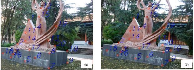 | |
| Fig. 10(a-b): | Matching results under different viewpoints |
CONCLUSIONS
Two algorithms of recovering camera motion parameters are proposed on the assumption that the camera has been calibrated. Algorithm 1 recovers the camera motion parameters from the essential matrix. Algorithm 2 recovers camera motion parameters by coplanarity equation. Algorithm 1 and 2 are commonly used in computer vision and photogrammetry, respectively. Comparatively speaking, the precision of Algorithm 1 is a little higher than Algorithm 2. However, Algorithm 1 requires eight pairs of matching points at least and considers the deterioration. Algorithm 2 only needs five pairs of matching points for recovering camera motion parameters. More importantly, Algorithm 2 doesn’t have the degenerate case, so Algorithm 2 is more suitable. In this study, the derivation of two algorithms is revealed in detail. Finally, simulation and real experiments results show that the two algorithms are feasible and very close. Meanwhile, two algorithms also have the higher robustness and can satisfy the requirements of 3D reconstruction.
ACKNOWLEDGMENTS
This study is supported by the Natural Foundation of Yunnan Province, China (2011FB017), the Scientific Research Foundation of Yunnan Education Department of China (2010Y245) and the Scientific Research Foundation of Yunnan University (2010YB021).
REFERENCES
- Elatta, A.Y., L.P. Gen, F.L. Zhi, Y. Daoyuan and L. Fei, 2004. An overview of robot calibration. Inform. Technol. J., 3: 74-78.
CrossRefDirect Link - Hartley, R.I., 1997. In defense of the eight-point algorithm. IEEE Trans. Pattern Anal. Mach. Intell., 19: 580-593.
Direct Link - Kaawaase, K.S., F. Chi, J. Shuhong and Q.B. Ji, 2011. A review on selected target tracking algorithms. Inform. Technol. J., 10: 691-702.
CrossRefDirect Link - Longuet-Higgins, H.C., 1981. A computer algorithm for reconstructing a scene from two projections. Nature, 293: 133-135.
CrossRefDirect Link - Luong, Q.T. and O.D. Fraugeras, 1997. Self-calibration of a moving camera from point correspondences and fundamental matrices. Int. J. Comput. Vision, 22: 261-289.
CrossRef - Yakar, M., H.M. Yilmaz, S.A. Gulec and M. Korumaz, 2009. Advantage of digital close range photogrammetry in drawing of muqarnas in architecture. Inform. Technol. J., 8: 202-207.
CrossRefDirect Link - Murthy, G.R.S. and R.S. Jadon, 2011. Computer vision based human computer interaction. J. Artif. Intell., 4: 245-256.
CrossRefDirect Link - Hussain, S., V.S. Giridhar, P.C. Reddy and K. Kumari, 2007. Implications of minimum markers in the segmented watershed images. Inform. Technol. J., 6: 1158-1161.
CrossRefDirect Link - Wang, S., J. Wang and Y. Zhao, 2009. A linear solving method for rank 2 fundamental matrix of non-compulsory constraint. Proceedings of the IEEE International Conference on Robotics and Biomimetics (ROBIO), December 19-23, 2009, Guilin, pp: 2102-2107.
CrossRef - Guo, Y., Y. Gu and Y. Zhang, 2011. Invariant feature point based ICP with the RANSAC for 3D registration. Inform. Technol. J., 10: 276-284.
CrossRefDirect Link - Pu, Y.R., S.H. Lee and C.L. Kuo, 2011. Calibration of the camera used in a questionnaire input system by computer vision. Inform. Technol. J., 10: 1717-1724.
CrossRef - Zhang, Z., R. Deriche, O. Faugeras and Q.T. Luong, 1995. A robust technique for matching two uncalibrated images through the recovery of the unknown epipolar geometry. Artif. Intell., 78: 87-119.
CrossRef - Zhang, Z., 2000. A flexible new technique for camera calibration. IEEE Trans. Pattern Anal. Mach. Intell., 22: 1330-1334.
Direct Link - Zhao, Y. and X.D. Lv, 2012. An approach for camera self-calibration using vanishing-line. Inform. Technol. J., 11: 276-282.
CrossRefDirect Link