
Emad A. Az-Zo`bi
Department of Mathematics and Statistics, Mutah University, Mutah, P.O. Box 7, Jordan
Trends in Applied Sciences Research
Year: 2015 | Volume: 10 | Issue: 3 | Page No.: 157-165


ABSTRACT
In this study, the Variational Iteration Method (VIM) is considered for solving systems of conservation laws with source terms. This method is based on the use of Lagrange multipliers; it changes the differential equation to a recurrence sequence of functions whose limit is considered as the solution of differential equation. The convergence of this method for solving such equations is presented by introducing the sufficient conditions of convergence and an error estimate. Two examples with physical interests are investigated to verify the effectiveness and reliability of the VIM.
PDF Abstract XML References Citation
Received: December 14, 2014;
Accepted: April 14, 2015;
Published: May 08, 2015
How to cite this article
Emad A. Az-Zo`bi, 2015. On the Convergence of Variational Iteration Method for Solving Systems of Conservation Laws. Trends in Applied Sciences Research, 10: 157-165.
URL: https://scialert.net/abstract/?doi=tasr.2015.157.165
URL: https://scialert.net/abstract/?doi=tasr.2015.157.165
INTRODUCTION
Conservation laws are first order quasi-linear partial differential equations that arise in many physical models. They asserted that the rate of change of the total amount of substance contained in a fixed domain Ω is equal to the flux of that substance across the boundary of Ω plus the rate that the substance is created in Ω (Lax, 1987). In one space dimension, a scalar conservation law in two independent variables is of the form:
| (1) |
where, u is called the conserved quantity, f is the flux and h is the source term. The variable t denotes time, while x is the one-dimensional space variable.
In the last years, many mathematicians have devoted their attention to study solutions of this type of equations. Among these attempts are the finite difference method (Sod, 1978), the Sinc-Galerkin method (Alquran and Al-Khaled, 2011), Adomian Decomposition Method (ADM) (Alquran and Al-Khaled, 2011; Safari, 2011; Az-Zo'bi, 2014), Variational Iteration Method (VIM) (Raftari and Yildirim, 2012; Abdou and Soliman, 2005; Khatami et al., 2008), Homotopy analysis method (Khatami et al., 2008; Hosseini et al., 2010). Homotopy perturbation method (Mohyud-Din et al., 2010; Berberler and Yildirim, 2009) and the Reduced differential transform method (Az-Zo'bi and Al-Dawoud, 2014).
In order to study convergence of the VIM for solving nonlinear system of conservation laws, the sufficient conditions and error bounds are addressed. New illustrating examples have been investigated to verify convergence results.
MATERIALS AND METHODS
Variational iteration method: The VIM was first proposed by the Chinese mathematician He in 1999 as modification of a general Lagrange multiplier method (Inokuti et al., 1978) for solving a wide range of problems whose mathematical models yield differential equations or systems of differential equations. The VIM has successfully been applied to many situations. It was shown by many authors that variational iteration technique is efficient and powerful in solving ordinary, partial and integro-differential equations of both fractional and natural orders (Wazwaz, 2014a, b; Wang et al., 2014; Mishra and Saini, 2014; Akkouche et al., 2014; He et al., 2014; Khaleel, 2014; Neamah, 2014). In this part, this approach was presented to handle the system of conservation laws (Eq. 1):
Consider the n-th-dimensional system of conservation laws:
| (2) |
For i = 1, 2,..., n, subject to initial conditions:
| (3) |
To illustrate the basic concepts of VIM, for = 1, 2,..., n, the n-th-dimensional system of conservation laws in the operator form was considered:
| (4) |
Subject to initial conditions:
| (5) |
Where:
are linear differential operators. The initial value problem in Eq. 3 and 4 can be written in more compact form as:
| (6) |
where, U = (u1,..., un)T, the vector function F = (f1,..., fn)T is nonlinear operator called the fluxes terms and H = (h1,..., hn)T is the source terms.
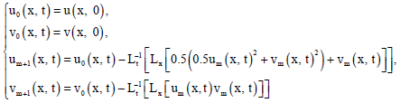
According to VIM, a correction function can be constructed as follows:
| (7) |
Where:
is considered as a restricted variations, i.e.![]() = 0 and the subscript m denotes the m-th order approximation. Λ(τ) is the vector of optimal values of the generalized Lagrange multipliers λi(τ), i = 1, 2, ..., n, which can be identified optimally via the variational theory by using the stationary conditions, with respect to Un, in the following form:
= 0 and the subscript m denotes the m-th order approximation. Λ(τ) is the vector of optimal values of the generalized Lagrange multipliers λi(τ), i = 1, 2, ..., n, which can be identified optimally via the variational theory by using the stationary conditions, with respect to Un, in the following form:
| (8) |
Thus, the stationary conditions are found in the form:
| (9) |
| (10) |
Which shows that all entries of the vector Λ are -1.
Substituting the identified Lagrange multiplier into Eq. 6 results in the following iteration formulation:
| (11) |
We start with an initial approximation U(x, 0) = G(x). The exact solution is given by:
| (12) |
Convergence analysis: The convergence of the VIM was discussed for linear and nonlinear differential equations in many works (Odibat, 2010; Sweilam and Khader, 2010; Ghorbani and Nadjafi, 2010). According to fixed point theorem, the sufficient conditions for convergence of the sequence solution in Eq. 11 is proved and the maximum absolute error is estimated.
Theorem 1: Let Um ε(C1 (R))n be the solutions of the sequence Eq. 11 obtained by VIM. Suppose, in addition, that the nonlinear operator F has Lipchitzian partial derivative in x with Lipchitz constant L. That is:
Then, for any bounded starting data U0 and a constant 0<γ = LT<1, the sequence {Um} converges to the exact solution (say U) of system in Eq. 6.
Proof: It can be seen that the sequence {Um} is a Cauchy sequence which has a unique limit in the Banach space (C1(R))n. Let, Uk and Um be two solutions of the sequence in Eq. 11 with k≥m, then:
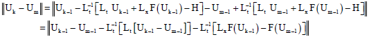 |
Since Uk(x, 0) = G (x) for all k and by Lipchitzian of Lx we get:
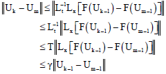 |
Consequently and since ||U1-U0||≤γ||U0||, we get:
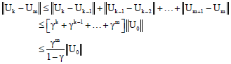 |
With 0<γ<1 and ||U0||<∞:
||Uk-Um||60 as m→∞ |
Thus, {Uk} is Cauchy sequence. To prove the coincide of the unique limit and exact solution of Eq. 6, we show that:
| (13) |
By continuity of LxF:
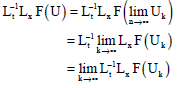 |
The proof is complete.
Theorem 2: Suppose that the hypotheses of Theorem 1 are satisfied, then the bounds for the error involved in using Um(x, t) to approximate the exact solution U(x, t) is given by for all:
Proof: It is obvious from Theorem 1.
RESULTS AND DISCUSSION
In this section computational results are presented. The mentioned technique is applied to various systems of conservation laws to illustrate the convergence of VIM discussed in previous section.
In materials and methods section, we show that the convergence sufficient conditions of the VIM for solving system of conservation law are strictly the contraction of the partial derivative flux term and the boundedness of the source term. So, examples with known solutions allow for more complete error analysis. For those with unknown solutions, an error bound can be computed using Theorem 2.
Example 1: Consider the Cauchy problem (Az-Zo’bi and Al-Khaled, 2010):
| (14) |
With the initial data:
| (15) |
The system in Eq. 14 is of mixed-type whose exact solution is:
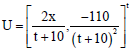 | (16) |
Applying the VIM, the iteration equation (Eq. 11) for system (Eq. 14) can be constructed as:
 | (17) |
The obtained solution follows closed exact solution form Eq. 16 as more and more successive approximations computed. On some domain R = (-α, α)×[0,1], ![]() ,the flux term has contraction partial derivative in variable x with γu = 0.19 and γv = 0.28. Theorem 2 implies that the truncated solutions of degree m≥1 have error bounds:
,the flux term has contraction partial derivative in variable x with γu = 0.19 and γv = 0.28. Theorem 2 implies that the truncated solutions of degree m≥1 have error bounds:
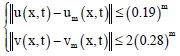 | (18) |
In this example, the solutions start outside the elliptic region, afterwards enter this region for some finite x and t. The finite difference method (Holden et al., 1990) showed unstable solutions inside elliptic region. On the other hand, the Adomian approach (Az-Zo’bi and Al-Khaled, 2010) and the VIM are stable and convergence while Cauchy problem (Eq. 14) changes type with faster convergence in variational iteration case.
Example 2: Consider the p-system (Az-Zo’bi, 2013):
| (19) |
That describes the one-dimensional longitudinal motion in elastic bars or fluids, where u is the velocity, v is the specific volume and p is the pressure. A well-known example of p-system is a van der Waals fluid whose pressure is given by:
| (20) |
where, R is the gas constant, T is the temperature, a and b are positive constants. With RT = 1, a = 0.9 and b = 0.25. We discuss this problem with smooth initial conditions for ![]()
| (21) |
The exact solutions of Van der Waals equations are unknown, so absolute errors in comparison to exact solutions can’t be determined. Instead, approximate fluid velocity and volume were computed using three iterations of Eq. 11 and error bounds are estimated using Theorem 2 as:
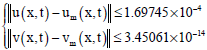 | (22) |
The fluxes have stepwise contraction partial derivatives in the given domain up to m = 2, that is:
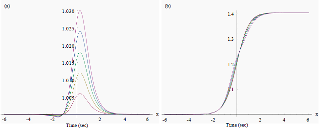 | |
| Fig. 1(a-b): | Numerical results for (a) Velocity u (x, t) and (b) Volume v (x, t) obtained at times t = 0, 0.4, 0.8,..., 2 |
So, the VIM is convergent. Unusually, the approximate solutions can’t be made more converge as more and more iterations are computed for m≥3, the fluxes will be unbounded and the solutions are diverge. Figure 1 shows different profiles of the obtained approximate solutions of u(x, t) and v(x, t), respectively.
As in the previous example, The Van der Waals system is of mixed type. In comparison to the ADM (Az-Zo’bi, 2013), the VIM shows graphically more stability and faster convergence.
CONCLUSION
The He’s variational iteration technique for solving systems of conservation laws is presented in addition to sufficient conditions that guarantee the convergence. This method is very powerful tool for solving these types of equations. Two mixed type examples were considered to illustrate the convergence study. The consistency of the variational iteration method can be obtained since the method is stable, while the system changes its type, as well as convergence. With unknown exact solutions, an error bound for mth order approximate solutions can be determined. The computations in this study were performed with aid of Mathematica.
REFERENCES
- Abdou, M.A. and A.A. Soliman, 2005. New applications of variational iteration method. Phys. D: Nonlinear Phenomena, 211: 1-8.
CrossRefDirect Link - Akkouche, A., A. Maidi and M. Aidene, 2014. Optimal control of partial differential equations based on the variational iteration method. Comput. Math. Applic., 68: 622-631.
CrossRef - Alquran, M.T. and K.M. Al-Khaled, 2011. Numerical comparison of methods for solving systems of conservation laws of mixed type. Int. J. Math. Anal., 5: 35-47.
Direct Link - Az-Zo'bi, E.A. and K. Al-Khaled, 2010. A new convergence proof of the Adomian decomposition method for a mixed hyperbolic elliptic system of conservation laws. Applied Math. Comput., 217: 4248-4256.
CrossRef - Az-Zo'bi, E.A., 2013. Construction of solutions for mixed hyperbolic elliptic Riemann initial value system of conservation laws. Applied Math. Modell., 37: 6018-6024.
CrossRef - Az-Zo'bi, E.A., 2014. An approximate analytic solution for isentropic flow by an inviscid gas model. Arch. Mech., 66: 203-212.
Direct Link - Az-Zo'bi, E.A. and K. Al-Dawoud, 2014. Semi-analytic solutions to Riemann problem for one-dimensional gas dynamics. Scient. Res. Essays, 9: 880-884.
CrossRefDirect Link - Berberler, M.E. and A. Yildirim, 2009. He's homotopy perturbation method for solving the shock wave equation. Applicable Anal., 88: 997-1004.
CrossRef - Ghorbani, A. and J.S. Nadjafi, 2010. Convergence of He's variational iteration method for nonlinear oscillators. Nonlinear Sci. Lett. A: Math. Phys. Mech., 1: 379-384.
Direct Link - He, J.H., 1999. Variational iteration method: A kind of non-linear analytical technique: Some examples. Int. J. Non-Linear Mech., 34: 699-708.
CrossRef - He, J.H., H.Y. Kong, R.X. Chen, M.S. Hu and Q.L. Chen, 2014. Variational iteration method for Bratu-like equation arising in electrospinning. Carbohydr. Polym., 105: 229-230.
CrossRef - Holden, H., L. Holden and N.H. Risebro, 1990. Some Qualitative Properties of 2x2 Systems of Conservation Laws of Mixed Type. In: Nonlinear Evolution Equations that Change Type, Keyfitz, B.L. and M. Shearer (Eds.)., Springer-Verlag, New York, pp: 67-78.
Direct Link - Hosseini, M.M., S.T. Mohyud-Din, S.M. Hosseini and M. Heydari, 2010. Study on hyperbolic telegraph equations by using homotopy analysis method. Stud. Nonlinear Sci., 1: 50-56.
Direct Link - Khaleel, O.I., 2014. Variational iteration method for solving multi-fractional integro differential equations. Iraqi J. Sci., 55: 1086-1094.
Direct Link - Khatami, I., N. Tolou, J. Mahmoudi and M. Rezvani, 2008. Application of homotopy analysis method and variational iteration method for shock wave equation. J. Applied Sci., 8: 848-853.
CrossRefDirect Link - Mishra, H.K. and S. Saini, 2014. Variational iteration method for a singular perturbation boundary value problems. Am. J. Numer. Anal., 2: 102-106.
Direct Link - Mohyud-Din, S.T., A. Yildirim and G. Demirli, 2010. Traveling wave solutions of Whitham-Broer-Kaup equations by homotopy perturbation method. J. King Saud Univ. Sci., 22: 173-176.
CrossRef - Neamah, A.A., 2014. Local fractional variational iteration method for solving volterra integro-differential equations within local fractional operators. J. Math. Stat., 10: 401-407.
CrossRef - Odibat, Z.M., 2010. A study on the convergence of variational iteration method. Math. Comput. Modell., 51: 1181-1192.
CrossRef - Raftari, B. and A. Yildirim, 2012. Analytical solution of second-order hyperbolic telegraph equation by variational iteration and homotopy perturbation methods. Results Math., 61: 13-28.
CrossRef - Safari, M., 2011. Analytical solution of two extended model equations for shallow water waves by Adomian's decomposition method. Adv. Pure Math., 1: 238-242.
CrossRefDirect Link - Sod, G.A., 1978. A survey of several finite difference methods for systems of nonlinear hyperbolic conservation laws. J. Comput. Phys., 27: 1-31.
CrossRef - Sweilam, N.H. and M.M. Khader, 2010. On the convergence of variational iteration method for nonlinear coupled system of partial differential equations. Int. J. Comput. Math., 87: 1120-1130.
CrossRef - Wang, G.Y., J.H. He and L.F. Mo, 2014. Variational iteration method for nonlinear oscillators: A comment on application of Laplace iteration method to study of nonlinear vibration of laminated composite plates. Latin Am. J. Solids Struct., 11: 344-347.
CrossRef - Wazwaz, A.M., 2014. The variational iteration method for solving linear and nonlinear ODEs and scientific models with variable coefficients. Central Eur. J. Eng., 4: 64-71.
CrossRefDirect Link - Wazwaz, A.M., 2014. The variational iteration method for solving new fourth-order emden-fowler type equations. Chem. Eng. Commun., (In Press).
CrossRefDirect Link