
R. Derakhshani
Department of Geology, Shahid Bahonar University, Kerman, Iran
A. Bazregar
Sangab Zagros Consulting Engineers, Shiraz, Iran
Trends in Applied Sciences Research
Year: 2010 | Volume: 5 | Issue: 1 | Page No.: 48-55


ABSTRACT
The effective solute transport parameters, longitudinal dispersivity (αx), transversal dispersivity (αy) and retardation factor (R) for a two-dimensional plume are estimated using time-concentration data of a sampling borehole through which the plume passes. The plume was produced by injection of 2 kg Uranine (Sodiumfluorescien; Color Index: 45350) in a borehole in uniform groundwater flow. Two-dimensional analytic equation of solute transport in a uniform groundwater flow was used to estimate the parameters. The results were compared with one well method of dispersivity estimation. A time-concentration curve was drawn using estimated parameters and compared with the observed time-concentration curve. Comparison shows the accuracy of the estimated parameters obtained by the former method. Based on the estimated parameters and the two-dimensional analytic equation the movement of the plume is predictable at any arbitrary time after injection for the study area. Based on the estimated parameters and the two-dimensional analytic equation the movement of the plume is predicted at 85 days after injection for the study area, where as it is shown in this study the predictable and observed concentration curve are exactly equal.
PDF Abstract XML References Citation
How to cite this article
R. Derakhshani and A. Bazregar, 2010. Estimation of Two Dimensional Solute Transport Parameters Using Tracing Experiment Data. Trends in Applied Sciences Research, 5: 48-55.
URL: https://scialert.net/abstract/?doi=tasr.2010.48.55
URL: https://scialert.net/abstract/?doi=tasr.2010.48.55
INTRODUCTION
Dispersivity parameters are needed for prediction of movement of a contaminant and can be estimated in the field by two general methods. The first method involves measurement of a real contaminant plume that exists in the field and the second method involves injection of a tracer in the aquifer. The latter is a much more common approach for determining dispersivities than using an existing contaminant (Zou and Parr, 1994). Local transverse dispersion was lionized as an important factor in the controlling the rate of dilution of conservative solutes and smoothing of concentration fluctuations (Fiori and Dagan, 2000). Local transverse dispersion transfers longitudinal spreading of solute plumes to effective mixing in heterogeneous media (Dentz et al., 2000; Cirpka and Kitanidis, 2000; Cirpka, 2002; Benekos et al., 2006). Chen et al. (2005), Cirpka and Kitanidis (2001) and Benekos et al. (2006) proposed some methods for determination transverse dispersivity. Benekos et al. (2006) and Cirpka and Kitanidis (2001) introduced a method to estimate the transverse dispersion coefficient by best fitting breakthrough curves with numerical simulations. Transverse dispersion coefficient was determined from net rate of nonaqueous phase liquid pool dissolution by Eberhardt and Grathwohl (2002). Cirpka et al. (2006) estimated transverse dispersion coefficient by measuring plume length of alkaline plume in acidic ambient while Klenk and Grathwohl (2002) have studied transverse vertical dispersion in groundwater, by using the results of experiments on mass transfer of volatile compound across the capillary fringe. More recently, Massabo et al. (2007) introduced a quick method for the laboratory-scale estimation of the transverse dispersion coefficient which was based on the analytical solution of the advection-dispersion equation where a pulse-like injection of a nonreactive solute was conducted in a column packed with a homogeneous porous medium.
MATERIALS AND METHODS
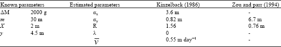
This study which was conducted in 2008 is concentrated on estimation of two dimensional solute transport parameters using tracing experiment data in Korbal plain, situated in South of Iran. Two estimation methods are used in the present paper in which transport parameters can be estimated for a two-dimensional plume generated by a slug tracer injection in a uniform ground water flow field. In the first method, the two-dimensional advection-dispersion equation of Kinzelbach (1986) is employed by which the longitudinal and transversal dispersivity parameters were determined using an observed time- concentration curve in a sampling well.
In the second method, one well method of dispersivity estimation of Zou and Parr (1994) is used to estimate these parameters.
RESULTS
The field tracing experiment was conducted in the Korbal plain, situated in South of Iran, 55 km North-West of the city of Shiraz (Lat.: 29°, 30. Lon.: 52°, 45). Nearest mountain to the Korbal plain that highly has affected the geology and hydrogeology of the plain, is Rahmat anticline with the N-W to S-E trend corresponds to the Zagros ranges trend. The Zagros fold-thrust belt, which extends for about 2000 km from Southeastern Turkey through Northern Syria and Iraq to Western and Southern Iran, with its numerous supergiant hydrocarbon fields, is the most resource-prolific fold thrust belt of the world (Derakhshani and Farhoudi, 2005; Sepehr and Cosgrove, 2004). This fold and thrust belt is a result of the structural deformation of the Zagros (peripheral) proforeland system, whose present-day expression is the marine Persian Gulf and continental Mesopotamia basins and underlying preproforeland, mostly platformal and continental shelf deposits (Alavi, 2004). The belt has structurally evolved as a prism of stacked thrust sheets, composed of uppermost Neoproterozoic and Phanerozoic sedimentary strata approximately 7 to 12 km thick, in the external part of the southwest-migrating Zagros orogenic wedge (Alavi, 1994). More than a hundred stratigraphic columns have been studied from both subcrop (well) and outcrop (measured) sections in various parts of the Zagros belt (Alavi, 2004; Rahnama et al., 2008; Bahroudi and Koyi, 2004; Adabi et al., 2008; Ghavidel-syooki and Vecoli, 2008; Fakhari et al., 2008; Shirazi, 2008).
The dominant formation of Rahmat anticline is Sarvak (L. Cretaceous, Limestone) and in some area along the anticline axes at the crest, the Kazhdumi Formation (Albian-Cenomanian, shale and marly limestone) is exposed (Fig. 1). Eroded material of this Formation has produced fine texture sediment of the study area. The soil texture in the study area is reported to be silty-clay with 30% prosity and thickness of that is about 30 m. The groundwater flow velocity is very slow. The general direction of flow is down dip from the
 | |
| Fig. 1: | Geologic map and borehole positions in study area |
North-West towards the South-East (along the Rahmat anticline foot). However, the groundwater flow direction in the tracing site in the time of experiment was exactly determined using several borehole data dug for this purpose. The location of the boreholes and direction of local groundwater is shown in Fig. 1.
It is assumed that a constant linear velocity for a uniform saturated groundwater flow field exists and that the tracer is conservative and the diffusion component of hydrodynamic dispersion is ignored. The advection-dispersion equation for a conservative solute in these conditions is:
| (1) |
where, c is mass of solute per unit volume of solution, x and y is Cartesian coordinates, t is time, ![]() is liner velocity of field flow in the x direction, αx and αy are dispersivities in the x and y directions.
is liner velocity of field flow in the x direction, αx and αy are dispersivities in the x and y directions.
The instantaneous input of a mass ΔM of solute as a vertical line source at x and y in a uniform infinite flow field results in a two dimensional plume which is derived from Eq. 1 and described by Kinzelbach (1986) as follows:
| (2) |
Where:
| m | = | Is aquifer thickness |
| ne | = | Effective porosity |
| R | = | Retardation factor |
| λ | = | Is a decay constant |
DISCUSSION
Eleven boreholes with depth of about 20 m and diameter of 10 cm were dug in the experiment site, as it is shown in Fig. 1. The bore hole I is used as injecting point which 2 kg of Uranine mixed with 50 L of water was injected into it (Fig. 1). Other 10 surrounding bore holes (W1, S1, S2 …) were used as sampling point which they were sampled for a period of 162 days. The Uranine was detected and measured in the samples by the means of a Shimadzu RF 5000 spectro-fluorophotometer with a sensitivity of 0.001 ppb.
Due to the fine texture of the soil in the experiment site, the flow velocity was very low and dye was detected in only two sampling boreholes, E1 and S1 (Fig. 1). The time-concentration curves for these two bore holes are shown in Fig. 2. Due to some limitations and the low velocity of groundwater, the time-concentration curve for sampling bore hole E1 was not completed. Therefore, the observed time-concentration curve of S1 was used to estimate the solute transport parameters.
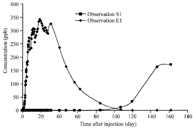 | |
| Fig. 2: | Observed time-concentration curve of boreholes S1 and E1 |
The two-dimensional solute transport equation of Kinzelbach (1986) was used to estimate the effective parameters based on the minimum differences between observed data and analytic data produced by Eq. 2. The results are given in Table 1 using observed data of sampling bore hole (S1) with Cartesian coordinates of x = 2 m and y = 4.5 m. Analytic time-concentration curve using estimated parameters is shown and compared with the observed curve in Fig. 3. These curves are close enough to prove that the estimated values are greatly close to the real values of the field characteristics. In Fig. 3, the observed and analytic curves cross each other at the point of 85 days after injection. It shows that at this time, the estimated concentration have the most agreement with the field measured data.
Dispersivity for a two dimensional plume can be determined by several methods such as one well method, two well method, areal method and inverse method. In this experiment, because there is available only one sampling well that, time-concentration data is complete, therefore, one sampling well method of dispersivity estimation (Zou and Parr, 1994), is used to compare with the first method explained above. One sampling well method requires concentration versus time data from one sampling well through which the plum passes. In order to determine the transversal dispersivity, the observation well should be off the plume centerline. This method is an extension of the two-well method proposed by Zou and Parr (1993). Equations that used for calculation of longitudinal and transversal dispersivity, given by Zou and Parr (1994) are as bellow:
| (3) |
| (4) |
| (5) |
| (6) |
where, R1 = cmaxtmax/ cltl and cmax and tmax are concentration and related time of maximum concentration in time-concentration curve. C1 is the half of the maximum concentration cmax/2 and t1 is the time of c1.
These equations are used to calculate αx and αy when ![]() and the plume direction are known. According to above equations and observed time-concentration of borehole S1, dispersivities are estimated as: αx = 6.7 m and αy = 0.76 m. Table 1 shows the estimated parameters from these two methods for comparison. The known parameters are presented also in Table 1 too.
and the plume direction are known. According to above equations and observed time-concentration of borehole S1, dispersivities are estimated as: αx = 6.7 m and αy = 0.76 m. Table 1 shows the estimated parameters from these two methods for comparison. The known parameters are presented also in Table 1 too.
It is obvious that the Zou and Parr (1994) method only uses two pairs of time-concentration data to estimate the dispersivitis coefficient. Also, by this method other parameters like λ and R cannot be estimated. In order to examine the accuracy of the dispersivity coefficients observation and analytic time-concentration curve based on parameters given by Zou and Parr (1994) method is shown in Fig. 4.
| Table 1: | Estimated solute transport parameters from Kinzelbach (1986) and Zou and Parr (1994). Known parameters used in parameter estimation are given too |
 | |
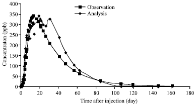 | |
| Fig. 3: | Observation and estimated time-concentration curve of borehole S1 using parameters derived from Kinzelbach (1986) |
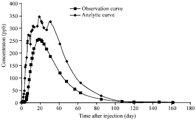 | |
| Fig. 4: | Observation and estimated time-concentration curve of borehole S1 using parameters derived from Zou and Parr (1994) |
Comparison of Fig. 3 and 4 show the accuracy of dispersivity estimation using the Kinzelbach (1986) equation. Therefore, parameters that can be given by this method are more reliable and were used to predict the plume concentration in groundwater system in the study area.
CONCLUSIONS
The accuracy of the estimated parameters obtained by the two-dimensional analytic equation of solute transport in a uniform groundwater flow method is demonstrated in the study area. Based on the estimated parameters and the two-dimensional analytic equation, the movement of the plume is predictable at any arbitrary time after injection for the study area. Movement of the plume is predicted at 85 days after injection for the study area and as it is shown in this paper the predicted and the observed concentration curves are exactly equal.
ACKNOWLEDGMENTS
The authors would like to extend their thanks to Dr. Zare for his useful suggestions. The authors greatly appreciate the scientific comments of Dr. Raeisi. We appreciate the critical reading by the arbitration committee and we welcome any enlightening suggestions and insightful comments.
REFERENCES
- Adabi, M.H., A. Zohdi, A. Ghabeishavi and H. Amiri-Bakhtiyar, 2008. Applications of nummulitids and other larger benthic foraminifera in depositional environment and sequence stratigraphy: An example from the Eocene deposits in Zagros Basin, SW Iran. Facies, 54: 499-512.
CrossRef - Alavi, M., 2004. Regional stratigraphy of the Zagros fold-thrust belt of Iran and its proforeland evolution. Am. J. Sci., 304: 1-20.
CrossRefDirect Link - Alavi, M., 1994. Tectonics of the Zagros Orogenic belt of Iran: New data and interpretations. Tectonophysics, 229: 211-238.
CrossRefDirect Link - Bahroudi, A. and H.A. Koyi, 2004. Tectono-sedimentary framework of the Gachsaran Formation in the Zagros foreland basin. Marin Petroleum Geol., 21: 1295-1310.
CrossRefDirect Link - Benekos, D., O.A. Cirpka and P.K. Kitanidis, 2006. Experimental determination of transverse dispersivity in a helix and a cochlea. Water Resour. Res., 42: 7406-7407.
CrossRef - Chen, J.S., C.W. Liu and C.P. Liang, 2005. Evaluation of longitudinal and transverse dispersivities distance ratios for tracer test in a radially convergent flow field with scale-dependent dispersion. Adv. Water Resour., 27: 887-898.
CrossRef - Cirpka, O.A. and P.K. Kitanidis, 2001. Theoretical basis for the measurement of local transverse dispersion in isotropic porous media. Water Resour. Res., 37: 243-252.
Direct Link - Cirpka, O.A., and P. K. Kitanidis, 2000. Characterization of mixing and dilution in heterogeneous aquifers by means of local temporal moments. Water Resour. Res., 36: 1221-1236.
Direct Link - Cirpka, O.A., 2002. Choice of dispersion coefficients in reactive transport calculations on smoothed fields. J. Contam. Hydrol., 58: 261-282.
CrossRef - Cirpka, O.A., A. Olsson, Q. Ju, M.A. Rahman and P. Grathwohl, 2006. Determination of transverse dispersion coefficients from reactive plume lengths. Ground Water, 44: 212-221.
CrossRef - Dentz, M., H. Kinzelbach, S. Attinger and W. Kinzelbach, 2000. Temporal behavior of a solute cloud in a heterogeneous porous medium: 1. Pointlike injection. Water Resour. Res., 36: 3591-3604.
CrossRefDirect Link - Derakhshani, R. and G. Farhoudi, 2005. Existence of the oman line in the empty quarter of Saudi Arabia and its continuation in the red sea. J. Applied Sci., 5: 745-752.
CrossRefDirect Link - Eberhardt, C. and P. Grathwohl, 2002. Time scales of organic contaminant dissolution from complex source zones: Coal tar pools vs. blobs. J. Contam. Hydrol., 59: 45-66.
PubMed - Fakhari M.D., G.J. Axen, B.K. Horton, J. Hassanzadeh and A. Amini, 2008. Revised age of proximal deposits in the Zagros foreland basin and implications for Cenozoic evolution of the High Zagros. Tectonophysics, 451: 170-185.
CrossRef - Fiori, A. and G. Dagan, 2000. Concentration fluctuations in aquifer transport: A rigorous first-order solution and applications. J. Contam. Hydrol., 45: 139-163.
CrossRef - Ghavidel-syooki, M. and M. Vecoli, 2008. Palynostratigraphy of Middle Cambrian to lowermost Ordovician stratal sequences in the High Zagros Mountains, southern Iran: Regional stratigraphic implications, and palaeobiogeographic significance. Rev. Palaeobot. Palynol., 150: 97-114.
CrossRef - Klenk, I.D. and P. Grathwohl 2002. Transverse vertical dispersion in groundwater and the capillary fringe. J. Contam. Hydrol., 58: 111-128.
CrossRef - Massabo, M., F. Catania and O. Paladino, 2007. A new method for laboratory estimation of the transverse dispersion coefficient. Ground Water, 45: 339-347.
CrossRef - Rahnama, R.J., R. Derakhshani, G. Farhoudi and H. Ghorbani, 2008. Basement faults and their relationships to salt plugs in the arabian platform in Southern Iran. J. Applied Sci., 8: 3235-3241.
Direct Link - Sepehr, M. and J.W. Cosgrove, 2004. Structural framework of the zagros fold-thrust belt, Iran. Marine Petroleum Geol., 21: 829-843.
CrossRefDirect Link - Zou, S. and A. Parr, 1993. Estimation of Dispersion Parameters for Tow-Dimensional Plumes. Groundwater, 31: 389-392.
CrossRef - Zou, S. and A. Parr, 1994. Two-Dimensional Dispersivity Estimation Using Tracer Experiment Data. Groundwater, 32: 367-373.
CrossRef