
Heshmatollah Askari-Hemmat
Department of Animal Sciences, Shahid Bahonar University of Kerman, Bahman 22 Boulevard, Kerman, Iran
Pakistan Journal of Biological Sciences
Year: 2006 | Volume: 9 | Issue: 12 | Page No.: 2189-2197


ABSTRACT
A new bio-economic deterministic approach and two crossbreeding simulation models i.e., the Stable model (ST) and the Variable model (VR) for 10 years of overlapping generations were developed. In the ST, the flocks’ size and system is stable and in the VR these may vary, as necessary. There are up to 3 flocks of 2 sire and dam breeds. A computer program examines all combinations to find the optimal system and flocks’ structure applying cash flow discounting. Each model proposes one or other of the rotational-, rota-terminal-, two way- and terminal-crossing systems under a detailed year-by-year approach, diagrammatically. The models were compared using the data attributed to the Australian Merino and Border Leicester. The ST required more ewes at the start and resulted in a higher cumulative net profit per ewe. It had less variation in the meat quality by use of generation preference and better utilization of breed effects due to less variation in the meatier breed’s gene contribution and to the stable flocks’ size. The VR needed more ewes to be as profitable as the ST in the end. Nonetheless, with same initial numbers of ewes for both models, the VR totally gained more profit due to a larger cumulative number of the ewes raised. Further, in the VR, the meat quality was unstable and there was too much delay in gaining a notable annual net profit. However, where there are low initial investments and limited resources available at the commencement of crossbreeding, the VR would be more suitable.
PDF Abstract XML References Citation
How to cite this article
Heshmatollah Askari-Hemmat, 2006. A Year-by-year Event Scheduled Simulation Approach to the Design of Meat Sheep Crossbreeding Systems. Pakistan Journal of Biological Sciences, 9: 2189-2197.
DOI: 10.3923/pjbs.2006.2189.2197
URL: https://scialert.net/abstract/?doi=pjbs.2006.2189.2197
DOI: 10.3923/pjbs.2006.2189.2197
URL: https://scialert.net/abstract/?doi=pjbs.2006.2189.2197
INTRODUCTION
The question of the optimal design for a lamb-producing crossing system is worth considerable attention. Simulation modelling is a major tool in this respect and studies of this nature can be used to address specific questions in animal breeding, as (Bourdon and Brinks, 1987) various genotype-management-environment-economic combinations can be tested at relatively low cost in a short time. It offers potential for more detailed and mechanistic understanding of the interface between breeding and production (Harris and Newman, 1994). There are two basic approaches to evaluating program design consequences; deterministic and stochastic (Kinghorn, 1993). The former generally, leads to the same result by running replicate programs and make a unique prediction for each set of the inputs without any associated internal variation and the latter contains random elements to predict the expected value of model performance variables and their dispersion as well (Pomar et al., 1991). Hence, employment of this approach results in variance in performance variables around the prediction.
An example of simulation modelling in sheep is a static and deterministic PC program called CS developed by Saviky (1993). The model predicts the performances, the population structure and the economic efficiency for an established population at equilibrium in terms of size and genetic composition. Similar computer programs for optimization of flock structures are usually designed, assuming that the related populations are at demographic equilibrium with a large number of animals and established gene frequencies. Another simulation program is ODCE - Optimum Design of Crossbreeding Experiments, developed by the BOKU (2004) to optimize designs for crossbreeding experiments. It specifies which genetic groups to use with how many observations in order to get maximum information about the set of specified crossbreeding parameters. The ODCE has an advantage over the CS etc., in that, it takes into account the intrinsic unbalancedness of crossbreeding designs due to the time effect over several generations. However, it lacks a detailed, year-by-year, graphically presentation for successive generations of crossbreeding.
The objective of this study was to develop a deterministic simulation approach with two computer simulation models to identify, for any appropriate set of the user-input data, a crossbreeding system for self-contained meat sheep enterprises, which would 1. be the most suitable system with two breeds in up to 3 flocks, 2. have the optimal flocks’ structure e.g., the optimal number of the ewes etc. in each flock, 3. be helpful to recognize the two-breed choice of the available breeds for crossing purposes, 4. benefit from taking into account the cash flow discounting effect on the economic consequences, as necessary.
This study uses 1) a totally new year-by-year approach with 10 years of overlapping generations, 2) two dynamic models i.e., the Stable model (ST) and the Variable model with cash flow discounting method, applying the above approach, all developed in this study and 3) two worked examples of these 2 simulation models for comparison. Two series of algorithm have been written for 2 computer programs which search all possibilities to recognize the choice for any given set of appropriate input data with arbitrary values. The computer programs require the phenotypic, the genetic and the management input parameters adding up to 27, including the biological traits. The optimal flocks’ structure and most of the important phenotypic, genotypic and economic parameters with the genetic composition of the flocks and other outputs are displayed diagrammatically for a clear understanding of the simulation modelling. Each model may propose one or the other of the rotational-, rota-terminal-, two way- and terminal-crossing systems, as an optimal case for any given set of the inputs depending on the inputs’ value.
MATERIALS AND METHODS
Methodology: In practice, many questions arise, regarding the details of the previous stages of breeding. For instance, what should be the age structure of the flocks at the start and later stages, how long does it take for a crossbreeding system to get established in terms of the expected population structure and breeds’ gene contribution. As regards the rotational systems, how long does it take to reach the equilibrium, what are the gene flow and the economics of the proposed system before equilibrium. Furthermore, how should we start to crossbreed to get the flocks ready for the proposed system at equilibrium and finally, what is the annual trend of the genetic and economic consequences for the proposed mating systems etc. Thus, practically before equilibrium, there is a great deal of the details commonly not outlined or graphically presented in the simulation modelling.
As stochastic approach is not very conductive to implementation in decision-aid software (Kinghorn, 1993), a deterministic approach to developing the models i.e., the Stable and the Variable models was employed in this study, to address such issues as above. These models were examined applying the standard cash flow discounting procedure (optional). In the Stable model, number of the ewes in each flock and, type of the crossing system is stable in all years throughout but, in the Variable, these may vary from one year to another. By means of these models, the breeder can recognize the 2-breed choice of the available sire and dam sheep breeds to use in up 3 flocks for crossbreeding with the optimal population structure and highest profitability possible. The models are aimed at the maximal cumulative (discounted) net profit in the final year, which correspondingly maximizes the cumulative (discounted) net profit for the previous years as well. Thus, the optimal annual number of the replacement ewe hoggets, the ewes and the slaughter lambs etc., for each flock are computed by use of the aforementioned models, based on the phenotypic and genetic make-up of the related flocks, applying the standard cash-flow discounting method (optional).
Prediction of the economic consequences based on the user-input data envisaged for 10 years of crossbreeding with overlapping generations including year -1 and year 0 (as the preparatory years), up to year 8. Two sets of the algorithm for the models have been developed to identify the optimal numbers of different classes of the animals as well as the genetic composition and some other outputs for each flock and year.
A minimum generation interval of 2 years was assumed for the dam breed in the models; 19 months for the first mating of the ewe hoggets and 5 months for conception length. In an attempt to reduce the practical difficulties associated with crossing of sheep breeds, only 2 breeds of sheep and up to 3 flocks have been envisaged. As a general clue to help accelerate testing crosses of the candidate breeds, breed A should be a good dam breed with high prolificacy and mothering ability and breed B a superior sire breed with lambs of good carcass traits. As a result, complementarily between these types of breeds can be utilized.
The economic lifetime of the dam breed assumed 6 years. Therefore, the ewe replacement rates on the input data sheet are calculated as follows. As mentioned earlier, the dam breed ewes deliver their lambs at 2 years of age. It follows that as these ewes are sold at 6 years of age, therefore, the hogget ewes are replaced after 4 years. Accordingly, the ewe replacement rate for the dam breed has been envisaged 25%.
It was assumed that in year -1, proportion of the ewe hoggets (maidens) equals that of the replacement rate of the ewes and the whole complex of the sheep flocks is bought in, with the same proportion of the ewe hoggets. Thus, the proportion of the adult ewes in year -1 equals the survival rate of the dam breed ewes. All the adult and maiden ewes are conceived before purchase and, deliver their lambs at the beginning of the crossbreeding program, in year -1.
The numerical work: To predict the desired parameters and the flocks’ structure, the phenotypic and economic parameters together with the percent expression of heterosis, as a basic parameter, for separate reciprocal crosses have been used in the models.
In this study, the dominance model of heterosis in which breed dominance alone in crossbred, heterozygous animals is responsible for the expression of heterosis, has been employed. According to Kinghorn (1982), the level of heterozygosity between 2 purebred populations and crosses of them directly depends upon the level of heterozygosity with respect to breed-of-origin of genes. Breed dominance is greatest when all loci consist of two genes from different breeds as in a first cross. Other crosses show a proportion of heterosis equal to the proportion of gene pairs which are heterozygous with respect to breed of origin (Kinghorn, 1993). Hence, the expression of heterosis in the progeny directly depends upon the breed difference of their parents. Correspondingly, to compute the crossbred progeny traits performances, the amounts of heterosis have been derived using this concept and added to the mid parents’ performances, so that
| (1) |
where, PF1 represents the progeny’s expected performance, MP1 and MP2 parental mean performances, d breed difference and H, percent heterosis already obtained in a particular cross using purebred animals. In the more complicated cases, the performance of the flocks for each trait has been predicted based on the generalized equation below. It has been assumed that there are 2 breeds of sheep; breed X and breed Y. Also, the replacements for flock 1 are provided from flocks 1 and 2 of the previous year and are mated to the rams of breed X in flock 1. It follows that:
Mean performance of a flock for a particular trait = total proportion of the replacements
| * | {proportion of the replacements from flock 1 |
| * | [mean performance of breed X |
| + | (gene proportion of breed X in the flock |
| * | performance of breed X |
| + | gene proportion of breed Y in the flock |
| * | performance of breed Y)] / 2 |
| * | (1 + breed difference of the replacements in comparison with the sire breed used in the existing flock |
| * | proportion of heterosis resulting from the X*Y cross) |
| + | proportion of replacements from flock 2 |
| * | [mean performance of breed X |
| + | (gene proportion of breed X in the flock |
| * | performance of breed X |
| + | gene proportion of breed Y in the flock |
| * | performance of breed Y)] / 2 |
| * | (1 + breed difference of the replacements in comparison with the sire breed used in the existing flock |
| * | proportion of heterosis resulting from the X*Y cross)} |
| + | proportion of the ewes survived coming from the previous year |
| * | performance of the same ewes.(2) |
It must be emphasized that, this method of computing the production performances relates to the progeny traits and the weaning rate after crossing. Practically, for computing the ewe trait performances in a particular year, a similar manner has been employed in the modelling algorithm but, with reference to both the previous year and the year before that for 3 flocks. This is because of the overlapping generations, making different age classes of the animals. This means that, for instance, the older ewes existing at present in a particular flock are survivals from the previous year. Also, the maidens (ewe hoggets) which are ready to deliver their lambs at the beginning of the present year and which are part of the present ewes’ populations as the annual replacements, are born 2 years previously in the flocks concerned. So, the corresponding costs are incorporated into the algorithm for 2 years; in the same year they are born and also in the year after that.
For optimization of the flocks’ structure and construction of the profit equation, the input and output parameters which include the costs and returns have been used as follows:
The input parameters: These consist of 27, including the biological traits, given to the models via the input data sheet, as follows: weaning rate of the ewes, weaning rate of the ewe hoggets, slaughter weight of the lambs, body weight of the cull-for-age ewes, ewe replacement rate, greasy fleece weight of the ewes, greasy fleece weight of the hoggets, greasy fleece weight of the yearlings, clean fleece weight:greasy fleece weight ratio (= yield), fiber diameter, ewe mortality, weaning to hogget mortality, weaning to slaughter mortality, costs of husbandry per ewe per year, costs of feed per ewe per year, costs of feed and husbandry per slaughter lamb, costs of feed and husbandry from birth to yearling, costs of feed and husbandry from yearling to hogget, costs of marketing per ewe, costs of wool harvesting and marketing, price of 1 kg of clean wool of 21 microns in diameter, extra price (negative and/or positive) per 1 kg of clean fleece for each micron deviating from 21 microns, price of purebred replacements for year -1 and year 0, price of purebred ewes for year -1, price of ewes per kg body weight, price per kilogram live weight of lambs, discount factor, total number of the ewes for commencement of the system and heterosis for the most important traits in the reciprocal crosses. These input parameters are given to each model’s program through a separate input data sheet.
The output parameters: The computer models predict the following: 1. The phenotypic parameters including the production performances of different traits, most important of which include: slaughter weight of the lambs, body weight of the ewes, greasy fleece weight, fiber diameter, weaning rate and ewe replacement rate. 2. The management parameters i.e., number of the ewes in the flocks, number and source flock of the replacements, number of the slaughter lambs, number of the salvage animals (implicitly) and, number of the losses. 3. The genetic parameters include: degree of heterozygosity, breed difference, gene proportion in the ewes and hoggets of the breed (usually) superior in meat production and each breed’s gene contribution in the slaughter lambs. 4. The economic consequences for the optimal system i.e., the cumulative discounted net profit applying the standard cash-flow discounting method (optional) for each economic year and other details relative to the economics of the proposed system.
The economics of the models: In breeding programs, establishment costs and ongoing costs come early but returns come typically much later (Kinghorn, 1994). From the economic standpoint, it is clear that there is an inflation rate for any currency which causes a reduction in the value of money in future. Different production programs have different costs and returns in each stage of production and in each economic year. Accordingly, due to interaction between the inflation rate and the comparable costs and returns, a proper comparison of the profitability of say, two production systems becomes a critical task. Therefore, if we are to compare some particular production systems, we have to standardize the corresponding costs and returns for each system. This is done by way of dividing all the related costs and returns by the annual inflation rate at the end of each economic year. Basically, cash-flow discounting is usually applied where two or more production systems or selection programs are to be compared.
Discounting gives a different perspective on the true value of the program. However, it usually delays the break-even point: raises the cost of initial input and lowers value of delayed returns (Kinghorn, 1994). To predict the cumulative discounted net profit in each year for the models, the discount factor 1/(1 + d)t from Nicholas (1987) has been incorporated into the models’ algorithm for cash flow discounting, where: d is discount rate and t, the unit of time, e.g., year.
The optimization procedure: The generalized instructions to observe in writing the algorithm for computer optimization of a population’s structure in a year-by-year, event scheduled scheme, as produced and exercised in this study are as follows: 1. Setting up the required equations accommodating all of the relationships between the flocks’ structure, the phenotypic and the genotypic parameters and the economic factors. 2. Determining numbers of the hoggets as regular replacements required for each flock as well as for the flocks in the next 2 years (because of a minimum of 2 years generation interval). 3. Computing numbers of the surviving ewes allowed remaining in the flocks concerned. If the model has a variable number of the ewes, propose additional numbers of the replacement hoggets and/or lessen number of the survivals (ewes) as well as that of the migrant hoggets, for the next year. 4. Nominating the relevant flocks in the second last year for providing the trial numbers of the hoggets. Also, in the present year, the flocks from which the proper numbers of hoggets for the next 2 years are supplied should be suggested. 5. Calculating number of the available female progeny as replacements in each flock. 6. Recommending some reasonable numbers of hoggets from the candidate flocks for the recipient flocks. 7. Solving the equations linked to and use the values of the variables adjusted to certain levels by computer program. 8. Repeating all the previous stages to search all possibilities to find the optimal population’s structural elements by changing the linked variables’ values through iteration using the algorithm. 9. Selecting the most profitable flocks’ structure considering the economic consequences for a certain time period. 10. Using a proper software with appropriate algorithm and a set of the initial arbitrary values for the linked variables, the computations for optimization of the flocks’ structure are relatively performed automatically, following the above rules.
The breeds’ characterization: The breeds used in the worked examples are the Australian Merino and Border Leicester. The Merino is suitable for wool production and is good in mothering ability. It is characterized by hardiness and can be used as a prime dam in crossbreeding programs. The Border Leicester is an English long wool breed and since its introduction to Australia has made an enormous contribution to the development of Australia’s Prime Lamb industry. This breed is good in twinning, milking, mothering ability, fast growth rate and valuable long wool attributes (Shands, 1987). Accordingly, the Merino has been used as a dam breed and the Border Leicester as a sire breed in the worked examples.
The input parameters in the worked examples: Most of the input parameters were obtained from Cottle (1991), Ponzoni (1986), Atkins (1987) and McGuirk (1978). Also, in addition to the derivation of values for a few parameters from intuition, in some cases reasonable assumptions in this regard were necessarily made, following consultation with the national LAMBPLAN Coordinator Prof. R. Banks and Mr. Allan Luff - N.S.W. Agr., Cawri, Australia.
RESULTS
The approach: Design of the year-by-year deterministic simulation approach for meat sheep crossbreeding plus two deterministic computer models i.e., the Stable and the Variable models has been accomplished and examined in this study. The approach with overlapping generations i.e., with different age classes of the sheep in each year, has been shown in Fig. 1. It is a simplified figure of a series of 10 consecutive flow charts, each presenting the details of one crossbreeding year for lamb producing enterprises.
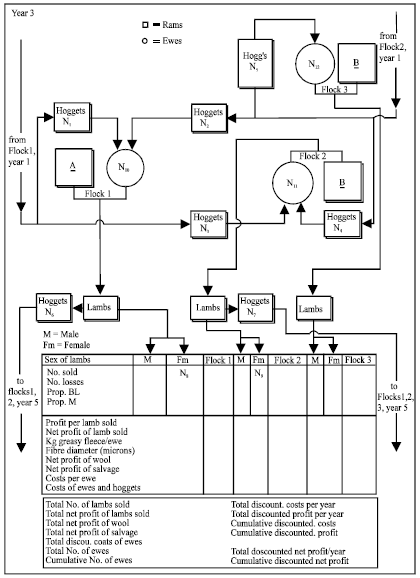 | |
| Fig. 1: | Part of the year-by-year approach and the population’s main structural elements i.e., the predictable Numbers N1-N12 of the migrant ewe hoggets and those of the slaughter female lambs and ewes in the flocks. Most of the predictable output parameters can be seen as well |
As described earlier, in the Stable model, the flocks’ size and type of the crossing system will not change throughout the course of crossbreeding program but, in the Variable model, these may vary from one year to another, whenever necessary (Fig. 2). Both of the models use a year-by-year approach for simulation.
The initial total number of the ewes to commence with, in year -1 (the first year), as an input datum, is optional. In both models, in year -1, numbers of the ewes in flocks 1 and 2 are determined from and add up to, the total number of the ewes required at start, by a computer program for the optimal structure and system of the flocks. This is fulfilled via adjusting the linked, adjustable Variables’ values incorporated into the algorithm, once the total initial number of the ewes has been specified by the breeder. Furthermore, in addition to separate annual flow charts, separate sets of the adjustable variables are allocated for different years. These are incorporated into a separate linked worksheet to facilitate the optimization process.
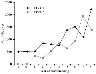 | |
| Fig. 2: | Variability of number of the ewes in the Variable model as occurred in the worked example |
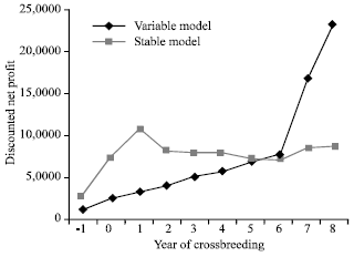 | |
| Fig. 3: | Trends of profit in the Stable and the Variable models-with cash flow discounting and same initial number of the ewes for both models |
Results of the worked examples of the models: With same sets of the inputs as described earlier, for both models, the Stable model proposed a rota-terminal and the Variable a combination rotational crossing system, the latter including some sub-systems.
The Variable model used different numbers of ewes in each year of crossbreeding, as presented in Fig. 2. It can be seen from Fig. 2 that, numbers of the ewes in both flocks fluctuated in various ways except that, these numbers remained unchanged from year -1 to year 1 and year -1 to year 0, for flocks 1 and 2, respectively.
For a proper comparison, the standard cash flow discounting method was applied to both models. Using same numbers of the ewes at start (500) in both models resulted in a very rapid increase in discounted net profit per year for the Variable model in the final two years, with gradual rise in the previous years. Conversely, in the Stable model, there was a steep rise in profit in the first 3 years, so that it peaked in year 1. Then, the annual profit had a marked downturn in year 2, leveled off for one year and, then continued to have a slow decline by year 6 with little increase thereafter (Fig. 3).
The cash flow discounting had no effect on the flocks’ structure with same initial numbers of the ewes but, it changed the general trend of the annual net profit slightly.
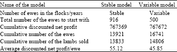
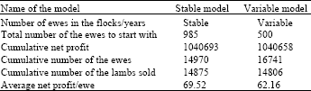
Next, both models were aimed at the same cumulative discounted net profit in the final year. So, the initial number of the ewes in the Variable model was held constant (500) and that in the Stable model was changed until both models’ cumulative discounted net profits in with-cash-flow-discounting procedure statistically equaled. Number of the ewes in year -1 in the Stable model (916) was worked out through different trials resulting in the same cumulative discounted net profit in year 8, for both models. Other outputs changed accordingly, some of which can be seen in Table 1.
As a result, the whole flocks’ structure had some changes i.e., the Stable model started with 916 ewes predicting 20.22% more cumulative net profit per ewe, owing to 16.85% fewer ewes raised and 6.57% fewer lambs sold, all compared to the Variable model.
| Table 1: | Different initial numbers of the ewes with same cumulative discounted net profits in year 8 envisaged for comparison of the worked examples of the models - with cash flow discounting |
 | |
There was almost a steady but, large rise in profit for the Stable model whereas that for the Variable model had an increasingly upward trend of gradual increase by year 6 in the form of a curve. From year 7 onward, there was a steep rise to the same cumulative discounted net profit as the Stable model’s ($A 767369), gained in year 8 (Fig. 4).
| Table 2: | Different initial numbers of the ewes and same cumulative net profits envisaged for comparison of the worked examples of the models - without cash flow discounting |
 | |
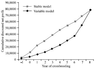 | |
| Fig. 4: | Trends of the annual cumulative discounted net profit for the Stable and the Variable models, with different ewe population sizes at the beginning but same final cumulative profit |
In a different experiment, without cash flow discounting, the same procedure as above was followed for the models. Part of the results has been presented in Table 2.
Consequently, the above mentioned figures for without-cash-flow-discounting procedure were 985 (13.8% larger), 8.38% smaller, 6.27% larger and 7.03% larger, respectively. Moreover, the initial number of the ewes was always higher for the Stable model; 83.2% higher in with- and 97% higher in without-cash-flow-discounting method, both with equal cumulative net profits.
DISCUSSION
Usually, the populations for which simulation programs are designed are not at equilibrium and it is assumed that there is a large number of the animals with established gene frequencies. This is a weakness of such modelling programs. Practically, in most conditions, the population size is small without equilibrium. Meanwhile, especially with crossbreeding programs, a great deal of differences exists between all the animals in different years of breeding in terms of breed composition, age group, performances etc., which results in various levels of overall profitability. In addition to the crossbreeding parameters, a time effect which may be called year, generation, mating round, etc, has often to be included in the reproduction of analysis. In many cases, especially if the experiment is conducted over several generations of crossbreeding, not all genetic groups e.g., third generation animals are available from the beginning of the experiment. This produces an intrinsic unbalancedness of the resulting design (BOKU, 2004). The year-by-year approach introduced in this paper deals with this issue by illustrating 10 separate genetic groups consisting of different age classes of animals. It presents the trends for different aspects of breeding and management of the flocks e.g., genetic composition, meatier breed’s gene contribution, economic evaluations and, flocks’ structure etc, in addition to type of the crossing system.
The functional aspects of the models: As can be seen from Fig. 1 (year 3), there are the predictable main numbers of the animals; N1-N12, based on which, the system and flocks’ structure of the enterprise are identified. Numbers of the migrant, replacement hoggets (N1-N5) and numbers of the ewes (N10-N12; only for the Variable model) are central to optimization of the flocks’ structure. Other numbers and the output parameters are affected by these numbers’ values i.e., numbers N6-N9 are determined indirectly once the Numbers N1-N5 (and N10-N12) specified by the models. At this stage, all of the output parameters can be computed. The main Numbers mentioned above determine how many of the female lambs should be sold and how many should be raised as hogget for replacement purposes in the corresponding flocks in the future.
The variation in the number of the ewes in the Variable model results from the possible use by the model of fewer ewes survived coming from the previous years, for a particular or all of the flocks in the next year, as necessary. In other words, even with any given stable replacement rates in different years in the Variable model, flocks’ size may change from one year to another for optimality.
In a Variable strategy (the Variable model), the linked variables’ values could vary from one year to another, while in a Stable strategy the same values are used in the equations concerned, every year. In prediction of the numbers, there is a set of the fixed elements as part of the algorithm in the equations, as well as a number of the aforementioned adjustable structural elements i.e., the adjustable parameters or linked variables determining the predictable numbers N1-N5 and N10-N12. In other words, these numbers are directly affected by the linked Variables adjustable for the optimal values which in turn, this results in the optimal system and flocks’ structure. This is done by iteratively searching all possible combinations for the linked variables by the related model’s computer program, in a separate worksheet. So, the optimal numbers of the migrant hoggets and the ewes are directly specified by automatically adjusting the linked Variables concerned. As a result, an optimum-design population structure resulting in the maximum profitability for the enterprise will be recognized.
It follows that, the numbers N1 + N3 = N6 for year 1 and N2 + N4 = N7 for the same year. This is because it has been assumed that the first mating of hoggets occurs at 19 months of age. Thus, the replacement hoggets are predestined from the relevant flocks 2 years previously. Meanwhile, N8 + N6 and N7 + N9 (plus number of the losses) add up to the total number of the lambs weaned in the flocks concerned.
If the Numbers N2 and N3 ≥ 1 and N5 = 0 → the system is a rotational crossing. When N2 and N3 ≥ 1 and N5 ≥ 1 → the system is a terminal-rotation crossing. Also, when N1 and N3 ≥ 1 and N2 = 0 → the system is a terminal crossing. The same will be for the situation in which N2 and N4 ≥ 1 and N3 = 0. Some other combinations may be proposed by the models as well.
Thus, at the beginning in year -1, the whole population of the sheep for the flocks should be purchased according to the numbers shown in the related diagrams. Prices of the purebred dam breed in year -1 and year 0 have been included in the models’ input data sheet. In other years, no hoggets are purchased but the costs, other than the purebreds’ are taken into account as part of the costs mentioned earlier. It must be noted that no replacement ewe hoggets but, all the purebred rams (or semen doses) are purchased from outside of the population.
Until end of year 3 (the fifth year) new algorithm has been used every year and, after that little alterations have been made in this respect. However, due to the numerous separate year-by-year illustrations as flow charts, with the corresponding linked variables for 10 years and, the too lengthy algorithm for both models (which would be useful to the reader only if viewed jointly), it is not possible to make a full presentation of them in this manuscript. Accordingly, due to the space limitation, it has been limited to the basic equation (2) and to the simplified Fig. 1 with adequate explanation.
In Fig. 1, the costs of the young hoggets born in year 3 with numbers of N6 and N7, which are predestined for year 5, are incorporated into both year 3 and year 4 (but not graphically presented in year 4), as costs of the hoggets and, costs of the ewe hoggets, respectively. Further, the performances of these animals affect the mean performance of the whole related ewe populations in year 5 (and similarly, this is true for any other year). Meanwhile, in each year, there are also some ewe hoggets that are being raised but, born in the year before that, delivering their lambs at the beginning of the next year. For instance, those born in year 2, with umbers of N6 and N7 in that same year, exist in year 3 (but not graphically presented in year 3), are to be used in year 4 as replacements for flocks 1 to 3, presented as N1-N5 in year 4.
Thus, the net profit of wool in a particular year has been computed considering all different age groups of the sheep, as pointed out above. As regards lamb production, the related performances are computed for the slaughter lambs just for the same year they are born, for they are sold or slaughtered shortly after weaning or, even when they are too younger.
CONCLUSIONS
To sum up briefly, the result of this study shows that, the event-scheduled year-by-year approach introduced in this manuscript helps improve bio-economic evaluation of crossbreeding designs and management of population structure, via illustration of the breeding system details and offering numerical values for different crossbreeding choices in a wide range of conditions.
As regards the worked examples of the models developed and examined in this study, it was found that, with same initial numbers of the ewes for both models, the Variable model had a sudden annual rise in profit in the final 2 years due to a larger cumulative number of the ewes raised. But, in terms of the overall profitability within any given period of time, with different initial ewe population sizes, the Variable model needed more cumulative number of ewes to be as profitable as the Stable model, i.e., same cumulative discounted net profit over a 10 year crossbreeding period.
In other words, with equal final cumulative discounted net profit for both models, the crossing system proposed by the Variable model produced a larger number of the salable lambs through retaining the crossbred female lambs in the flocks in order to propagate the ewes for a higher level of lamb production at the later stages of crossing. This caused a reduction in the average cumulative discounted net profit gained per ewe, due to the increased maternal costs for a larger number of the breeding ewes. Further, in the Variable model, the meat quality was unstable and there was too much delay in gaining a notable annual net profit.
For a particular cumulative amount of discounted net profit in year 8, the Stable model required more ewes at the beginning but, resulted in a higher cumulative discounted net profit per ewe. It had less variation in the meat quality by use of generation preference and better utilization of the breed effects. This is due to less variation in the meatier breed’s gene contribution and to the stable flocks’ size for the Stable model. However, where there are low initial investments and limited resources available at the commencement of crossbreeding, the Variable model would be more suitable.
ACKNOWLEDGMENTS
The author wishes to thank Prof. B.P. Kinghorn - The Univ. of New England: For his advice, Prof. M.E. Goddard - AGBU: For his valuable initial ideas regarding optimal crossbreeding designs, Prof. R. Banks - LAMBPLAN coordinator and, Mr. Allan Luff-Livestock officer of N.S.W. Agr., Cowri, Australia: For their assistance in the collection of the input data and the MSRT of Islamic republic of Iran for the financial support.
REFERENCES
- McGuirk, B.J., 1978. Effects on survival and growth of first-cross lambs and on wool body measurements of hogget ewes. Aust. J. Exp. Agric. Husbandry, 18: 753-763.
CrossRef - Pomar, C., D.L. Harris, P. Savoie and F. Minvielle, 1991. Computer simulation model of swine production systems III. A dynamic herd simulation model including reproduction. J. Anim. Sci., 69: 2822-2836.
Direct Link