
M. Frikha
Ecole Nationale d�Ingenieurs de Sfax, �ENIS�, Department of Genie Electrique, BP W, 3038, SFAX, Tunisia
Z. Ben Messaoud
Ecole Nationale d�Ingenieurs de Sfax, �ENIS�, Department of Genie Electrique, BP W, 3038, SFAX, Tunisia
A. Ben Hamida
Ecole Nationale d�Ingenieurs de Sfax, �ENIS�, Department of Genie Electrique, BP W, 3038, SFAX, Tunisia
Journal of Applied Sciences
Year: 2007 | Volume: 7 | Issue: 24 | Page No.: 3891-3899


ABSTRACT
This study investigates the issue of improving the discriminative training capabilities in Hidden Markov Model (HMM) isolated word recognition task. Hence for, two optimization criterions in the training phase are focused; the minimization of recognition Word Error Rate (WER) according to the Baum-Welch based Maximum Likelihood Linear Estimation (MLE) and the Maximum Likelihood Linear Regression (MLLR) adaptation training criterion. For this purpose, the Statistical Learning Theory (SLT) and the MLLR adaptation are applied in order to analyze, in the sense of minimum word error rate, the consistency of the training estimator in clean and mismatched environmental conditions. Several experiments were carried out. They all aimed to find an efficient training estimator algorithm with good generalization property and allowing a good training error rate with a significant training data reduction. The obtained results show that it exists an optimal specified training conditions which should be reached in order to guarantee an optimal discriminative training characteristics of the HMM based isolated word recognition system.
PDF Abstract XML References Citation
How to cite this article
M. Frikha, Z. Ben Messaoud and A. Ben Hamida, 2007. Towards Discriminative Training Estimators for HMM Speech Recognition System. Journal of Applied Sciences, 7: 3891-3899.
DOI: 10.3923/jas.2007.3891.3899
URL: https://scialert.net/abstract/?doi=jas.2007.3891.3899
DOI: 10.3923/jas.2007.3891.3899
URL: https://scialert.net/abstract/?doi=jas.2007.3891.3899
INTRODUCTION
Automatic Speech Recognition (ASR) is a pattern recognition problem. Statistical pattern recognition techniques have been successfully applied to many problems, including speech recognition. The majority of current automatic speech recognition systems employ statistical techniques to model speech (Ben-Yishai and Burshtein, 2004). The Hidden Markov Model (HMM) method is statistically based and its success has triggered a renewed urge for a better understanding of the traditional statistical pattern recognition approach to speech recognition problems. The advent of powerful computing devices and the success of Hidden Markov Modeling released a renewed pursuit for more powerful statistical methods to further reduce the recognition Word Error Rate (WER) and build more robust speech recognition systems across various conditions. The accuracy of state of the art recognition systems relies on properly trained parameters with minimum training data (Tong, 2001). That’s why a tremendous research work is actually intended on finding new Discriminative Training (DT) algorithms yielding to an increase of speech recognition accuracies in clean and noisy environments. Approaches to improve discrimination between confusable classes can be categorised in two ways. In the first category, discrimination is improved by operating the recogniser in a feature space in which the acoustic units of interest are inherently better separated. In a second category, the problem of discrimination is addressed at the model level by building better classifiers. Discriminatively-trained hidden Markov models fall under this category (Ben-Yishai and Burshtein, 2004; Juang and Katagiri, 1992).
The present research is motivated by the following observation; robust parameter estimates from insufficient training data is a research topic itself, then we intended to give an answer to the following question: how much training data do we need to be able to construct a good classifier? Of course, increasing the size of the database nearly always results in a decrease of error rate. The reason for this is that the more training data one has, the more parameters one can afford to train and, consequently, the more detailed the models can be. Unfortunately, the use of much training data, will result many drawbacks such that the increase of processing time, or other logistic difficulties.
So, we focused in this research study, an improvement, in the model training level, of the HMM recognition system described by Frikha et al. (2007). Our major concern was basically oriented on studying the efficiency of the training estimator by varying its capacity represented by the size of data as well as the complexity of the estimated function. So, we studied in this present research:
| • | The application of the Statistical Learning Theory (SLT) (Vapnik, 1999; Cherkassky and Malier, 1999; Ganapathiraju, 2002), which is a new paradigm for solving learning problems in, HMM speech recognition applied to the isolated word task. Our motivation of using such technique is that SLT is developed for small data samples and does not rely on a priori knowledge about the problem to be solved, in contrast to the classical statistics developed for large samples and based on using various types of a priori information. Therefore, SLT provides a new framework for the general learning problem. |
| • | The implementation of the Maximum Likelihood Linear Regression (MLLR) adaptation (Leggetter and Woodland, 1995; Lee and Huo, 2000), which has been recognized as an effective approach to overcome the mismatch between the training and testing conditions. MLLR was a transformation-based adaptation where the overall HMM were transformed via the cluster-dependent linear regression functions estimated by the Maximum Likelihood (ML) theory. In environmental adaptation, we attempt to transform the acoustic features means of a HMM so as to better match the characteristics of some speech from a particular environment. |
STATISTICAL SPEECH RECOGNITION OVERVIEW
A typical statistical speech-recognition system is shown in Fig.1. The goal in a statistically-based speech recognition system is to find the most likely word sequence given the acoustic data. If O is the acoustic evidence that is provided to the system and W = w1, …,wN is a sequence of words, then the recognition system must choose a word string ![]() that maximizes the probability that the word string W was spoken given that the acoustic data was observed (Rabiner, 1989):
that maximizes the probability that the word string W was spoken given that the acoustic data was observed (Rabiner, 1989):
| (1) |
P(W|O) is known as the a posteriori probability since it represents the probability of occurrence of a sequence of words after observing the acoustic signal. The above approach to speech recognition, where the word hypothesis is chosen within a probabilistic framework, is what makes most present recognizers statistical pattern recognition systems.
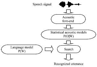 | |
| Fig. 1: | Schematic overview of a statistical speech recognition system |
It is difficult to directly compute the maximization of Eq. 1 since there are effectively an infinite number of word sequences for a given language from which the most likely word sequence needs to be chosen. This problem can be significantly simplified by applying a Bayesian approach to find (Rabiner, 1989):
| (2) |
The probability P(O|W), that the data was observed if a word sequence was spoken is typically provided by an acoustic model. The likelihood that gives the a priori chances of the word sequence being spoken is determined using a language model (Rabiner, 1989). Probabilities for word sequences are generated as a product of the acoustic and language model probabilities.
The process of combining these two probability scores and sorting through all plausible hypotheses to select the one with the maximum probability, or likelihood score, is called decoding or search.
Statistical Acoustic Modeling: Hidden Markov Modeling of Speech: In most current speech recognition systems, the acoustic modeling components of the recogniser are almost exclusively based on Hidden Markov Models (HMM).
HMM provide a statistical framework for modeling speech patterns using a Markov process that can be represented as a state machine. The temporal evolution of speech is modeled by an underlying Markov process (Rabiner, 1989). Hidden Markov modeling is a powerful statistical framework for time-varying quasi-stationary process and a popular choice for statistical modeling of speech signal.
Given a speech utterance, let O = (o1, o2.....oT) be a feature vector sequence extracted from the speech waveform, where ot denotes a short-time acoustic vector measurement. Further, consider a first-order N-state Markov chain governed by a state transition probability matrix A = [aij], where aij is the probability of making a transition from state i to state j. Assume that at t = 0 the state of the system q0 is specified by an initial state probability πi = P(q0 = i). Then, for any state sequence q = (q1, q2.....qT), the probability of q’s being generated by the Markov chain is:
| (3) |
Suppose the system, when at state qt, puts out an observation ot according to a distribution bq(ot) = P(ot|qt), qt = 1,2,.....,T. If we denote B the matrix containing the probability distribution in each state, B=[bjk], where bjk = P(ok|qt =j). Therefore, we can use the compact notation λ = (π, A, B) to fully define the HMM. The HMM used as a distribution for the speech utterance can then be defined as (Rabiner, 1989):
| (4) |
Where, bqt(ot) defines the distribution for short-time observations, this output probability distribution represents the probability of observing an input feature vector in a given state qt. At the core of the HMM is a Bayes classifier where classification is done using a simple likelihood ratio test. The output probability distribution could be parametrized in several ways. The most commonly used form of the output for continuous distribution is a multivariate Gaussian distribution.
Acoustic model estimation: The estimation of the parameters of the HMM acoustic models plays a vital role in the accuracy of the ASR system. A key to the widespread use of HMM to model speech can be attributed to the availability of efficient parameter estimation procedures (Rabiner, 1989; Baum, 1972). Maximum Likelihood Estimation (MLE) is one such optimisation criterion (Dempster et al., 1977). The motivation to use MLE comes from the probabilistic definition of the speech recognition process which attempts to find a word sequence which maximises a cost (likelihood) function: we should be able to estimate the model parameters λMLE = ![]() to maximise the probability of the observation sequence given the model (Saul and Rahim, 2002):
to maximise the probability of the observation sequence given the model (Saul and Rahim, 2002):
| (5) |
The Expectation-Maximisation (EM) algorithm provides an iterative framework for MLE (Dempster et al., 1977); given the structure of HMM and training data, the algorithm finds the parameter values of the HMM according to the maximum likelihood (ML) criterion.
In the EM algorithm, an auxiliary function ![]() is defined as:
is defined as:
| (6) |
The EM algorithm iteratively estimates a new parameter set ![]() by computing an auxiliary function
by computing an auxiliary function ![]() based on an old parameter set
based on an old parameter set ![]() (E-step) and then maximizing the auxiliary function over
(E-step) and then maximizing the auxiliary function over ![]() (M-step):
(M-step):
| (7) |
The convergence of this iterative procedure to a local maximum of the objective function is guaranteed (Baum, 1972; Dempster et al., 1977).
A speech recognizer trained by the ML criterion achieves good recognition rate only if training data are sufficient to estimate model parameters reliably and the modeling assumptions are correct. However, in reality, speech is not produced by a hidden Markov process and the training sample size is not large enough. In this situation, training by maximum likelihood estimation may not lead to the best possible model that maximizes the recognition rate (Juang et al., 1997). The maximum recognition rate may be indirectly achieved by separating different classes as much as possible.
STATISTICAL LEARNING THEORY
Supervised learning refers to learning from examples, in the form of input-output pairs (x,y), by which a system that isn’t programmed in advance can estimate an unknown function and predict its values for inputs outside the training set (Cherkassky and Malier, 1999; Tong, 2001).
The central issue of statistical supervised learning problem is presented as follows:
That’s have a set of measures D = {(xi, yi) εRn x {0,1}, i = 1,…,m} according to unknown jointed probability distribution P (x, y). F is a set of functions such that F = {fα(x)/αεΛ}.
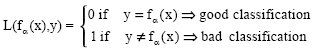
Our main objective is to find fα* ε F such that the estimation ![]() = fα*(x) will be the best possible. The choice of that function depends therefore on m training data iid according to the joint probability distribution P(x,y) = P(x).P(y|x). In order to select the function fα* from the given set of functions F, we need a loss function L(fα(x),y) which corresponds to the loss caused by using fα(x) to predict y. The traditional loss function for classification problems is (Vapnik, 1999):
= fα*(x) will be the best possible. The choice of that function depends therefore on m training data iid according to the joint probability distribution P(x,y) = P(x).P(y|x). In order to select the function fα* from the given set of functions F, we need a loss function L(fα(x),y) which corresponds to the loss caused by using fα(x) to predict y. The traditional loss function for classification problems is (Vapnik, 1999):
 | (8) |
Here, α is the generalized parameter of functions. Therefore, fα* will correspond to the function which minimizes the risk functional R(α) defined by Vapnik (1999):
| (9) |
In order to minimise the risk functional given by Eq. 9, for an unknown probability measure P(x,y). The expected risk functional is replaced by the empirical risk functional (or training error) which is constructed on the basis of the samples. This principle is called the Empirical Risk Minimization (ERM). The empirical risk functional is defined as (Vapnik, 1999).
| (10) |
Minimization of the above functional is one of the most commonly used optimization procedures in machine learning. ERM is computationally simpler than attempting to minimize the actual risk as defined in Eq. 10. Note that according to the law of large numbers:
| (11) |
This convergence is the main motivation for the Empirical Risk Minimisation (ERM): one hope that the function minimising the empirical risk (training error) will also have a small risk; then the ERM principle is said to be consistent.
Suppose we now receive a new set of data that does not include any of the examples used previously. For a machine that generalizes well, we should be able to predict with a high degree of confidence that the empirical risk obtained using this new data (or generalization error), will also be small. However this is not sufficient to guarantee a small generalization error. This phenomenon is called overfitting (Fig. 2).
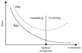 | |
| Fig. 2: | Underfitting and overfitting phenomena |
To avoid it, we need to restrict the class of functions on which the empirical error is minimized in order to have some guarantee on the efficiency of the algorithm.
This restriction to a prescribed set of functions called the model can lead to underfitting, i.e., to an estimator which has high empirical and expected risks. Therefore, to choose the adequate size (also called capacity or complexity) of the model is a key issue to build consistently efficient estimators. This implies that the expected risk (generalization error) tends towards the empirical risk. With this, we can guarantee both a small empirical risk (training error) and good generalisation with which we guarantee an ideal situation for a learning machine.
DISCRIMINATIVE ADAPTIVE TRAINING
Maximum-likelihood point estimation is by far the most prevailing training method. However, due to the problems of unknown speech distributions, such as sparse training data, high spectral and temporal variability of speech signal and possible mismatch between training and testing conditions, a dynamic training strategy is needed. To cope with the changing speakers and speaking conditions in real operational conditions for high-performance speech recognition, such paradigms incorporate a small amount of speaker and environment specific adaptation data into the training process. Bayesian adaptive learning is an optimal way to combine prior knowledge in an existing collection of general models with a new set of condition-specific adaptation data.
Maximum likelihood linear regression: Bayesian adaptive learning is an optimal way to combine prior knowledge in an existing collection of general models with a new set of condition-specific adaptation data. The most often used structure is through an affine transformation such as finding linear regression transformation of the mean vectors of the original HMM.
Maximum likelihood linear regression or MLLR computes a set of transformations that will reduce the mismatch between an initial model set and the adaptation data. More specifically MLLR is a model adaptation technique that estimates a set of linear transformations for the mean and variance parameters of a Gaussian mixture HMM system. The effect of these transformations is to shift the component means and alter the variances in the initial system so that each state in the HMM system is more likely to generate the adaptation data.
The transformation matrix used to get a new estimate of the adapted mean is given by Leggetter and Woodland (1995):
| (12) |
| (13) |
Where:
| W | = | N x(n + 1) transformation matrix |
| n | = | The dimensionality of the data) |
| ξ | = | The extended mean vector and w represents a bias offset |
Hence, W can be decomposed into:
| (14) |
Where:
| A | = | nxn transformation matrix |
| b | = | A bias vector |
The transformation matrix W is obtained by solving a maximisation problem using the Expectation- Maximisation (EM) technique (Bilmes, 1998). This technique is also used to compute the variance transformation matrix. The use of EM algorithm results a maximisation of a standard auxiliary function.
MLLR and regression classes: MLLR makes use of a regression class tree to group the Gaussians in the model set, so that the set of transformations to be estimated can be chosen according to the amount and type of adaptation data that is available (Leggetter and Woodland, 1995; Lee and Huo, 2000). The tying of each transformation across a number of mixture components makes it possible to adapt distributions for which there were no observations at all. With this process all models can be adapted and the adaptation process is dynamically refined when more adaptation data becomes available.
RESULTS
In all experiments we use the TIMIT database (DARPA, 1990). This corpus was designed for training and testing continuous speech recognition systems. The HTK toolkit (Young et al., 2002) was adopted for this study. The recognition system is a speaker independent isolated word recognition system developed to recognize 10 isolated words extracted from sa1 and sa2 testing and training corpus of TIMIT. The collected data was preprocessed using 25 ms Hamming window and a 10 ms frame period. Additionally, the data was preemphasized with a facteur of 0.97 and liftered with a factor of 24. For every frame we compute 12 Mel Frequency Cepstral Coefficients (MFCC) (Davis and Mermelstein, 1980). Those features were directly computed using standard HTK parametrisation module. Each vocabulary word was modeled by a five state left to right HMM with continuous Gaussian density associated to each state and no skip transitions. The training procedure involved initial estimates for word models followed by a five iteration of the Baum-Welch algorithm based on maximum likelihood estimation criterion. Recognition was then carried out using the Viterbi algorithm (Rabiner, 1989).
Series of experiments were conducted. They all aimed to find the optimal training complexity of the recognition system and this by searching the minimum Training Word Error Rate (TWER) and Generalized Word Error Rate (GWER) as well as the interval of confidence at 95% (IC95%) using Baum-Welch based MLE training criterion. It should be noticed that, the interval of confidence at x% from the recognition rate belongs to the interval [P-, P+], where (Barras, 1996):
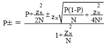 |
| (15) |
Where:
| P | = | The measured recognition rate |
| N | = | The number of realised tests |
| zx | = | A constant; it depends on the index x which indicates the percentage that the measured recognition rate is within the interval of confidence |
There is a chance of x% that the accurate recognition rate ![]() is within that interval. For large values of N, Eq. 15 may be further simplified and the recognition measurement error will be limited at 95% of the cases for example (Barras, 1996):
is within that interval. For large values of N, Eq. 15 may be further simplified and the recognition measurement error will be limited at 95% of the cases for example (Barras, 1996):
| (16) |
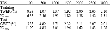
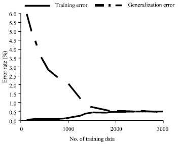
Experiment 1: For the first experiment, each acoustic vector was composed with 12 static MFCC coefficients. Each state was represented by a single multivariate Gaussian density with diagonal covariance matrix. In order to test the consistency of the training algorithm, based on MLE criterion, we gradually increase the Training Data Size (TDS). The Training Word Error Rate (TWER), generalisation word error rate (GWER) were measured and the interval of confidence at 95% (IC95%) was computed.
Table 1 shows the recognition performance measured in terms of training and generalised word error rate as a function of the size of training data. We observe that increasing the size of the training database will result in a decrease in the TWER up to certain optimal training data size (OTDS) of 2500 corresponding to a minimum word error rate of around 2%. We notice the relatively poor performance of the recognition system for small training data. This result is reasonably explained by Fig. 3. In fact, for small TDS, the recognition system is placed on the underfitting zone and therefore can not learn efficiently the model parameters. Above the OTDS, the recognition system is placed on the overfitting region conditions and its performance begins to fall down.
Experiment 2: The consistency of training algorithm depends on the complexity (number of estimated HMM parameters) of its mathematical function.
| Table 1: | Effect of variation of number of training data in error rate and confidence interval |
 | |
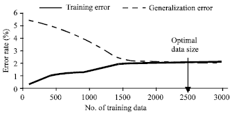 | |
| Fig. 3: | Consistency of the algorithm based on MLE criterion |
So, we studied in this second experiment the performance of the recognition system after varying its complexity by:
| • | Incorporating the dynamic features (first and second derivatives) to the static acoustic vectors. |
| • | Increasing the number of multivariate Gaussian mixtures of the acoustic models (HMM). |
Investigation of the incorporation of the dynamic acoustic features: The complexity is defined by the number of trained parameters:
| (17) |
Where:
| G | = | The number of Gaussian mixtures (G = 1 for this experiment) |
| N= 3 | = | The number of HMM emitting states and d is the dimension of coefficients |
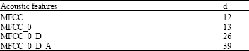
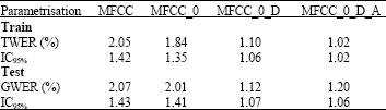
To illustrate the behaviour of the recognition system towards the increase of the complexity, we append the MFCC acoustic static features by their log energy ‘_E’ and first Δ ‘_D’ and second ΔΔ ‘_A’ order derivatives. Table 2 indicates the dimension of various kinds of acoustic features and Table 3 resumes the performance of the recognition system in terms of training and generalised word error rates as well as the interval of confidence at 95%.
| Table 2: | Dimension of different representations |
 | |
| Table 3: | Error rate and confidence interval when dynamic features appended |
 | |
 | |
| Fig. 4: | Effect of the incorporation of dynamic features on the performance of the recognition system |
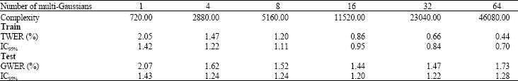
| Table 4: | Error rates and interval of confidence with different No. of Gaussian mixtures |
 | |
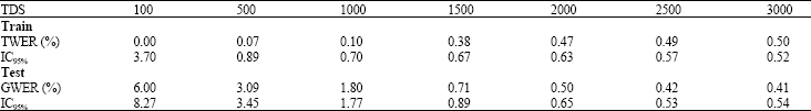
| Table 5: | Error rate and confidence interval with different number of training data |
 | |
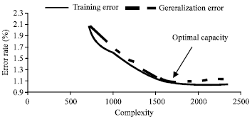
The obtained results are illustrated by the following curves displayed in Fig. 4. As can be seen, the incorporation of the time derivatives improved the performance of the recognition system but unfortunately at the price of an increase in complexity. This is in fact predictable since the time derivatives improve the ability between certain classes of sounds and some the temporal characteristics of speech signal (Furui, 1986).
From this experiment, the obtained Optimal Complexity (OC) of the recognition system corresponds to MFCC features appended by 0 order cepstral coefficient and first derivative coefficients. We also noticed the overfitting phenomena which appeared when exceeding the OC value.
Investigation of the increase of multivariate Gaussian mixtures: The recognition performance of the system is experimented while increasing the number of Gaussian mixtures in the output distribution (Table 4, Fig. 5).
As can be observed, the GWER decrease as the training data size grows (by increasing the number of Gaussian mixture per emitting state). A minimum GWER value of 1.44 is reached corresponding to an optimal complexity OC of 16 multivariate Gaussian mixtures per emitting state. The recognition system is put under the overfitting phenomenon after this optimal OC value.
Experiment 3: In this third experiment, we aimed to conduct the recognition system in the optimal condition obtained by the previous two experiments. So, the MFCC_0_D front end is used and 16 multivariate Gaussian mixtures were taken for each emitting state.
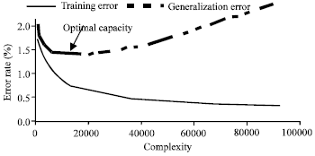
We evaluated the performance of the recognition system by gradually increasing the number of training data (Table 5, Fig. 6).
 | |
| Fig. 5: | Effect of the increase of gaussian mixtures on the performance of the recognition system |
 | |
| Fig. 6: | Consistence of the algorithm based on the MLE criterion |
Discussion: Optimal training data size OTDS of 2000 is reached for a corresponding generalised word error rate GWER of 0.5%. That means that a reduction of 500 in the vocabulary of the training data is obtained in comparison with results of the first experiment.
| Table 6: | Generalized word error rates and degradation for different values of SNR |
 | |
| Table 7: | Generalized error rate and gain with different size of adaptation data for different SNR values |
 | |
Substantial reduction in word error rate of 2% is obtained in comparison with the results of the first experiment.
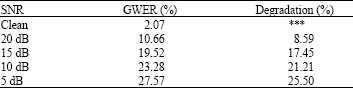
Experiment 4: The performance of automatic speech recognition systems is highly sensitive to variations between training and testing conditions. This experiment tries to study the influence of the mismatch between training and testing environment conditions. To do so, we add to our test signals an additive factory noise extracted from NOISEX-92 database (Varga et al., 1992) for different signal to noise ratio.
Table 6 shows the drastically degradation in the performance of the recognition system when deployed in an environment for which it has not been trained.
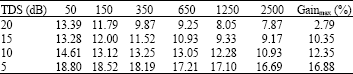
Investigation of MLLR adaptation technique: Model adaptation techniques have been shown as an effective way to address this problem of mismatch. The MLLR adaptation procedure works as the original training procedure to overcome this latter. We implemented MLLR algorithms for environment adaptation: Number of regression classes R was fixed to be four. We investigated the effect of the size of the adaptation data using the linear regression procedure.
The results collected from Table 7 show the performance of the adaptation process measured in terms of generalised word error rate as a function of the size of adaptation data.
We observe that the recognition performance increases with the size of adaptation data. However, a substantial gain in the WER of around 17% is reached for a SNR of 5 dB.
CONCLUSION
In this study, the Statistical Learning Theory (SLT) and the MLLR adaptation are applied in order to analyze, in the sense of minimum word error rate, the consistency of the training estimator based on MLE criterion in clean and mismatched environmental conditions. For this purpose, the issue of discrimination is addressed at the acoustic feature and model levels by building better classifiers yielding performing recognition system. Several experiments have been conducted for the purpose of finding the optimum training complexity according to the Baum-Welch based MLE training criterion. Followings are the essential of our findings.
In the first and second experiment, we showed that an optimal recognition system could be conceived with MFCC acoustic features appended by 0 order cepstral and first order derivatives, training data size of 2500 and 16 multivariate Gaussian mixtures associated to each emitting HMM state. The performance of the recognition system conducted in the optimal condition obtained by the previous two experiments is further evaluated in the third experiment by modifying the training data set. We observed that with only 2000 training data size, the generalized word error rate decreased by 2% in comparison with that obtained in the first experiment. We finally tested the MLLR adaptation algorithm of the recognition system tested in noisy environment. We clearly showed a great improvement of the recognition WER especially at low SNR values.
REFERENCES
- Ben-Yishai, A. and D. Burshtein, 2004. A discriminative training algorithm for hidden markov models. IEEE Trans. Speech Audio Process, 12: 204-217.
CrossRefDirect Link - Cherkassky, V. and F. Malier, 1999. Vapnik-chervonenkis (VC) learning theory and its applications. IEEE Trans. Neural Network, 10: 985-987.
CrossRefDirect Link - Davis, S. and P. Mermelstein, 1980. Comparison of parametric representations for monosyllabic word recognition in continuously spoken sentences. IEEE Trans. Acoust. Speech Signal Process., 28: 357-366.
CrossRefDirect Link - Dempster, A.P., N.M. Laird and D.B. Rubin, 1977. Maximum likelihood from incomplete data via the EM algorithm. J. R. Stat. Soc. Ser. B (Methodol.), 39: 1-38.
Direct Link - Juang, B.H., W. Chou and C.H. Lee, 1997. Minimum classification error rate methods for speech recognition. IEEE Trans. Speech Audio Processing, 5: 257-265.
CrossRefDirect Link - Lee, C.H. and Q. Huo, 2000. On adaptive decision rules and decision parameter adaptation for automatic speech recognition. Proc. IEEE., 88: 1241-1269.
CrossRefDirect Link - Leggetter, C.J. and P.C. Woodland, 1995. Maximum likelihood linear regression for speaker adaptation of continuous density hidden markov models. Comput. Speech Langanuage., 9: 171-185.
CrossRefDirect Link - Rabiner, L., 1989. A tutorial on hidden Markov models and selected applications in speech recognition. Proc. IEEE, 77: 257-286.
CrossRefDirect Link - Saul, L.K. and G. Rahim, 2000. Maximum minimum classification error factor analysis for automatic speech recognition. IEEE Trans. Speech Audio Proc., 8: 115-125.
Direct Link - Vapnik, V.N., 1999. An overview of statistical learning theory. IEEE Trans. Neural Networks, 10: 988-999.
CrossRefDirect Link