Weight-Based Feature Selection for Conditional Maximum Entropy Models

INTRODUCTION

Maximum Entropy (ME) models (Berger et al., 1996) have been widely used for many natural language processing tasks, including text classification, part-of-speech tagging and name entity recognition, etc. The models specify a probabilistic distribution over observed samples by defining a feature space (a set of features as well as their weights). Features are defined to be unconstrained arbitrary illustration of language phenomena in ME models and huge number of features could be generated using various methods. As a result, training a ME model would become intractable because of the huge memory needed. To solve this problem, two questions must be answered during the model building procedure: how to decide the usefulness of each feature and how to estimate the values of feature weights.

These two questions are often solved in two different manners: separately or jointly. In a separate manner, a feature selection procedure is first adopted with different strategies to obtain a useful feature set and then parameter estimation is taken place to determine the values of feature weights which express the importance of each feature. In the joint manner, parameter estimation is executed along with adding new features or deleting old features. It is much time and space saving to finish the feature selection before parameter estimation because the latter procedure is a quite time-consuming. However, it is hard to promise that the selecting strategies will satisfy the final need of applications. On the other hand, dealing with parameter estimation and feature selection jointly would take too much time especially the features are added or deleted one by one.

Many methods have been proposed for feature selection. Count Cutoff (Koeling, 2000) is the simplest and often used along with other methods. It only selects features occurring more than a predefined cutoff threshold times in the corpus. χ²-ranking (Chen and Rosenfeld, 1999) is another simple and effective technique. The χ²-test is computed using the count from prior and real training distribution, respectively. Mutual information (Yang and Pedersen, 1997) uses the dependency between a feature and its relevant class as the criteria and tends to select rarely occurred features. Incremental Feature Selection (IFS) algorithm (Berger et al., 1996) based on information gain provides a reasonable way to keep parameters of selected features unchanged when processing a newly added feature, but suffers from speed issues. To speed up this process, a φ-orthogonal condition (Berger and Printz, 1998) is proposed to select k features at the same time. This technique is efficient but the condition often fails when dealing with link features. Zhou and Wu (2003) used similar strategy but computed approximate gains for only top-ranked features based on models obtained from previous stages. Adaptive algorithms (Chen and Liginlal, 2008) are also implemented for feature selection and show superior performance.

The common ground of these methods is that features are judged based on different strategies before their weights are estimated. However, weights themselves should be the only factor to determine the importance of features. If the feature selection is put off until the final model is set up, then determining the importance of individual feature would become quite easy because weights are the right convincing evidence. To make this procedure practical, the feature set is first split into several subsets of moderate sizes. On each subset of features, a ME sub-model is trained. Feature selection based on weights is then implemented on these sub-models to choose useful features which are finally combined together to form the final ME model. The procedure could be repeated until the final model size is acceptable. Based on this idea, a weight-based feature selection algorithm is proposed. The task of part of speech tagging is employed as an example to show the performance of the method.

WEIGHT-BASED FEATURE SELECTION

ME models usually take the following probability distribution as its form:

(1)

where, f_i denotes the arbitrary feature to describe language phenomena, λ_i its corresponding weight and Z(x) the normalization factor (Berger et al., 1996).

A feature is composed of two parts: a predicate and a tag. The predicates are statements about the language phenomena and the tag is the category the observed object belongs to and will be predicted by the model. Features are often defined as binary functions that return 0 and 1 to indicate absence and presence respectively and weights are the determinative factor for calculating the probabilities. According to Eq. 1, features with weights close to zero act most likely as those absent. By carefully examination, we find out that this type of features take a major part of the feature space. If these features could be recognized in the feature space and removed, the model size would decrease hugely.

Suppose PRED denotes the set of all predicates to be examined. The training procedure of ME models can be shown as in Fig. 1. PRED is divided into several parts, with each part the training data is reconstructed and used to train a separated ME model. These sub-models define different feature spaces and have no common features between each other. Features are selected based on their weights in the sub-models and combined together to construct a new feature space, which could be used to restart the procedure or form the final model.

Fig. 1:	Training procedure based on weight-based feature selection. Describe the training procedure of ME models. Feature selection is used as a sub-module here. The main idea is to split feature space into several unrelated pieces, with each piece a sub-model is trained and its features are judged. Final model is constructed by combining sub-models together

To make the procedure work efficiently, the time and space consuming of each sub-model in step 2 of the algorithm should be restricted to a moderate degree. Suppose N is a suitable number of predicates on which the model could be built conveniently and |PRED| represents the size of original predicate set, then the value of m can be decided as:

(2)

Feature weights are a list of real numbers estimated by optimizing algorithms such as LBFGS (Liu and Nocedal, 1989) etc. By carefully examination on well-trained ME models, we find out that a large part of feature weights are close to zero, making their corresponding features take quite little role in determining the probability in Eq. 1. Present feature selection algorithm is trying to eliminate these features. Some held-out data is needed to measure the influence of eliminating features. Suppose evaluate is a function of some measure scales on held-out data (for example accuracy in following experiments). The feature selection algorithm is shown in Fig. 2.

The maximum and minimum weights should be found out in the beginning, denoted as MAX and MIN. MIN is often a negative number (if not, it will be set to 0). As the being examined weights are around zero, the boundaries of interval [NEGA, POSI] should be determined and shown in Fig. 3. Features with weights falling into this interval will be treated as useless and discarded to simplify the model.

Fig. 2:	Weight-based feature selection. Determine the interval boundary of feature weights. Features with weights in the interval are judged as useless and will be removed from the model. The examined interval is around zero

Fig. 3:	Intervals of feature weights; Describe the intervals determined by the feature weights of ME model. All feature weights are falling into [MIN, MAX] and features with weights in [NEGA, POSI] will be judged as useless and removed from ME mode

Binary search method (Knuth, 1997) is employed to determine the boundaries. The feature selection procedure tries to enlarge the range of [NEGA, POSI] where NEGA is the maximum negative weight boundary of features reserved to build final model and POSI is the minimum positive weight boundary. Take NEGA for example, its range [MINV, MAXV] is initialized as [MIN, 0]. During each of the iterations, NEGA is assigned to the middle value of MINV and MAXV and the features with weights in [NEGA, 0] are eliminated from the feature space to construct a new model. The interval [MINV, MAXV] is halved according to the loss by comparing with the original model. After several (10 in present experiments) iterations, NEGA takes MAXV as its final value. Similar procedure is performed to determine the value of POSI.

To judge if the loss on measure scales is acceptable or not, held out data and evaluation method should be given firstly. In present experiments, Accuracy is chosen as the evaluation criterion. A constant TOL (short for Tolerance) is given as the threshold to measure that if the loss is under control or not. The comparison result between TOL and the loss determine the direction of binary search. For example, when examining a certain NEGA, if the loss is less than TOL, the next search direction is left, otherwise the opposite. Its value is set to 0.01 in present algorithm.

EXPERIMENTS AND RESULT ANALYSIS

The chosen task for verification is part-of-speech tagging on English. Words and their gold part-of-speeches distributed in CoNLL 2008 shared task (Surdeanu et al., 2008) are used. There are 45 tags overall, Table 1 lists the data information.

The TRAIN and DEVEL datasets are used as training and held-out data respectively, BROWN and WSJ are used to test the ME models. To build the feature space, 7 templates (A-G) are employed to construct basic predicates. More predicates (H) are generated by combining different basic predicates in different positions surrounding current processing word. Table 2 shows the description.

These templates are implemented on training data and generate 16,929,090 predicates and 25,620,717 features. The two numbers could be reduced to 5,278,532 and 13,970,160, respectively by discarding predicates that appear only once in the training corpus. Figure 4 shows the distribution of feature occurrence from 1 to 1000. It is easy to find out that a majority of features occur rarely in the training data. In fact, there are 11,824,601 features appear no more than 5 times, take 84.64% of the feature space. On the other hand, only 16,547 features (take 0.11%) occur for over 1,000 times.

The maximum entropy modeling toolkit (http://maxent.sourceforge.net) is adopted to train ME models. For comparison and further examination, a benchmark model is trained using all the training data. The algorithms run on Solaris 9 Operating System for SPARC Platforms with 1200 MHz processer and 6 G memories. The training procedure takes about 11.23 h for 100 iterations.

All the feature weights are falling into [-2.0627, 4.2504]. The interval is averagely divided into 100 slices and the number of weights is counted for each slice. Figure 5 shows the distribution. Apparently, most of the features obtain weights around zero. In fact, 13,732,937 features have weights within [-0.0625, 0.0625], take 98.30% of the feature space.

Figure 6 shows the occurrence distributions of features that have weights internal and external of [-0.0625, 0.0625], indicated as internal and external, respectively. As can be seen, there are much more features of small weights (internal) than that of big weights (external) for a certain occurrence especially those features appearing for only a small number of times.Only occurrences from 1 to 500 are illustrated. When the occurrence is more than 500, the curves will become too wavy to be examined.

Table 1:	Information for training and testing data
Description of datasetsThe data are distributed on CoNLL 2008 shared task (Surdeanu et al., 2008)

Table 2:	Predicate templates
Description of predicates that are used to form features by combining with tags. A-G are basic predicates, H is generated by combining different basic predicates in different positions

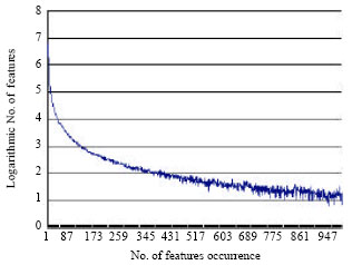Fig. 4:	Distribution of feature occurrence. The numbers of features occurring for certain times are counted on the feature space build on training dataset TRAIN. Features are defined in Table 2

Figure 7 gives the weight distributions of features appear more than 5 times and no more than 5 times, the weight interval is divided into 50 slices and for each slice, the number of features is counted. One interesting examination is that almost all the weights of features occurring no more than 5 times are smaller than 0.0625 and a majority part of them are around zero.

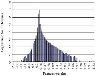Fig. 5:	Distribution of feature weights. The numbers of features with weights in certain small intervals are counted based on the ME model trained on the feature space without feature selection

Fig. 6:	Occurrence distributions for features. Data source is the ME model trained on the feature space without feature selection. Internal and External denote feature weights in and out of [-0.0625, 0.0625], respectively

Further examination shows that there are 11,799,766 features appearing no more than 5 times and having weights within [-0.0625, 0.0625], take 99.79% of features appearing no more than 5 times, 85.92% of features with weights in [-0.0625, 0.0625] and 84.46% of all features of the model. This could probably bring a conclusion that most (not all) rarely occurred features are useless. However, simply removing these features with a Cutoff method would probably miss some important features that occur rarely in the corpus. If the features are selected based on their weights, it can take the advantage of Cutoff method and also make reservation on useful features especially those important but rarely occurred.

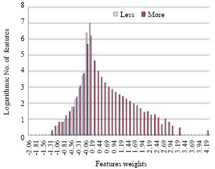Fig. 7:	Weight distributions for features occurring. Data source is the ME model trained on the feature space without feature selection. Less and More denote feature occurrences no more than and more than 5 times, respectively

Table 3:	Comparison between original model and present model
Comparison of different parameters between ME models. Original Model is the one without feature selection. Weight-based method denotes the model trained with present method

Following the algorithms described in Fig. 1 and 2, the predicate set of training data is randomly divided into 10 parts; with each part a sub-model is trained (200 iterations) and weight-based feature selection algorithm is implemented to find a useful feature space. These feature spaces are combined together to construct the final model. Table 3 shows the evaluation results on testing corpus.

The weight-based method outperforms the original model trained with all features on all three testing data DEVEL, BROWN and WSJ. Although, twice of the time has been used to implement the whole procedure, the number of features reduces to half of the original model. We can conclude that our method is feasible and efficient.

To make a comparison, the χ²-ranking method (Chen and Rosenfeld, 1999) is also implemented for feature selection. For each feature, the χ²-test is computed to judge the association between its predicate and tag. A ranking list is built based on the χ²-test values. The same number of features as our method are selected from the ranking list to train a ME model. The accuracies on DEVEL, BROWN and WSJ are 93.76, 88.41 and 94.20%, respectively, which are lower than the original model and present method.

Further examination shows that 3,392,018 (only 49.61%) common features are selected by the two feature selection methods, reflecting the difference between selection strategies.

REFERENCES

- Chen, Y. and D. Liginlal, 2008. A maximum entropy approach to feature selection in knowledge-based authentication. Decision Support Syst., 46: 388-398.
CrossRef - Chen, S.F. and R. Rosenfeld, 1999. Efficient sampling and feature selection in whole sentence maximum entropy language models. Proceedings of the Acoustics, Speech and Signal Processing, 1999 IEEE International Conference on ICASSP'99, March 15-19, 1999, Phoenix, Arizona, pp: 549-552.
Direct Link - Koeling, R., 2000. Chunking with maximum entropy models. Proceedings of the CoNLL-2000 and LLL, May 22, 2000, Lisbon, Portugal, pp: 139-141.
Direct Link - Liu, D.C. and J. Nocedal, 1989. On the limited memory BFGS method for large scale optimization. Math Program., 45: 503-528.
CrossRef - Zhou, Y.Q. and L.D. Wu, 2003. A fast algorithm for feature selection in conditional maximum entropy modeling. Theoretical Issues Natl. Language Process., 10: 153-159.
CrossRefDirect Link