A New Design of Active Noise Feedforward Control Systems Using Delta Rule Algorithm

INTRODUCTION

---

Active noises are real time noise and they cannot be predictable (i.e., random). The traditional way to cancel the noise, which is called passive noise control, which techniques based on the use of sound-absorbing materials, is effective in higher frequency noise. However, significant power of the industrial noise often occurs in the frequency range between 50-250 Hz. Here the wavelength of sound is too long, so that passive techniques are no longer cost effective because they require material that is too heavy.

Active Noise Control System is working based on the principle of superposition. The system consists of a controller for which reference about the noise is given. The controller properly scales the reference noise and the phase reverses it. The phase-reversed signal is then added to the input signal that has some noise along the original message signal so that the noise gets canceled out. There are many methods used for ANC system include both feedback and feed-forward control. ANC is based on either feed-forward control, where a coherent reference noise input is sensed before it propagates past the secondary source, or feedback control where the active noise controller attempts to cancel the noise without the benefit of an upstream reference input. The performance of the active control system is determined largely by the signal processing algorithm and the actual acoustical implementation. Effective algorithm design requires reasonable knowledge of algorithm behavior for the desired operating conditions. Since the active noise is random, the proper prediction of the noise cannot be possible, the controller should contain a adaptive filter part whose filter coefficients will be changing based on the error signal which the difference between the output of the controller and the output from an unknown plant. To achieve reduction of noise in complicated multiple noise source, we must use active noise control by multiple reference channel. That is input signal to the each channel is correlated and the output also correlated.

LMS ALGORITHM

The Least Mean Square, or LMS, (Douglas and Pan, 1995) algorithm is a stochastic gradient algorithm that iterates each tap weight in the filter in the direction of the gradient of the squared amplitude of an error signal with respect to that tap weight as shown in Fig. 1. The LMS algorithm is an approximation of the steepest descent algorithm which uses an instantaneous estimate of the gradient vector.

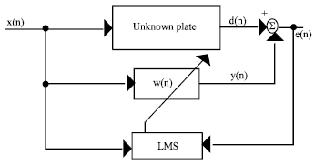Fig. 1:	Block diagram of the ANC control system using LMS algorithm

The estimate of the gradient is based on sample values of the tap input vector and an error signal. The algorithm iterates over each tap weight in the filter, moving it in the direction of the approximated gradient (Woo, 2001). Widrow and Hoff devised the LMS algorithm in 1959. The objective is to change (adapt) the coefficients of an FIR filter, w(n), to match as closely as possible to the response of an unknown system, p(n). The unknown system and the adapting filter process the same input signal x (n) and have outputs d(n) (also referred to as the desired signal) and y(n), respectively.

The LMS algorithm basically has two processes. The first one is the filtering process and the next is adaptive process. In filtering process, the reference signal is filtered in the adaptive filter and it is combined with desired signal. The error signal is the difference of the desired signal and the output signal of the filter w (n) (Glentis et al., 1999). In adaptive process, the reference signal and the error signal are fed to the LMS algorithm and the weights of the filter are modified based on the LMS algorithm.

It is assumed that all the impulse responses in this study are modeled by those of finite impulse response (FIR) filters. d(n) has the primary noise to be controlled and x(n) is the reference about the noise.

d(n) = pT(n) *x1(n)

(1)

where p(n) is the impulse response of the unknown plant and

x1(n) = [ x(n) x(n-1)...... x(n-M+1)]T

and M is the length of p(n). The y(n) is the output signal from the filter.

y(n) = wT(n) *x2(n)

(2)

where w(n) = [w(n) w(n-1) w(n-2)...YYw(n-N+1)]^T is the weight vector of the ANC controller with a length N and x₂(n)=[x(n) x(n-1)... .. x(n-N+1)]^T.

The error signal e(n) is difference of the desired signal d(n) and the output of the filter y(n).

e(n) = d (n)-y (n)

(3)

The weight of the filter w(n) is updated using the following equation;

w (n+1) = w(n) + x(n) e(n)

(4)

The termed as step size. This step size has a profound effect on the convergence behavior of the LMS algorithm. If is too small, the algorithm will take an extraordinary amount of time to converge. When is increased, the algorithm converges more quickly however, if is increased too much, the algorithm will actually diverge. A good upper bound on the value of is 2/3 over the sum of the eigen values of the autocorrelation matrix of the input signal. The correction that is applied in updating the old estimate of the coefficient vector is based on the instantaneous sample value of the tap-input vector and the error signal.

The correction applied to the previous estimate consists of the product of three factors: The (scalar) step-size parameter, the error signal the correction applied to the previous estimate consists of the product of three factors: the (scalar) step-size parameter, the error signal e(n-1) and the tap-input vector u(n-1). The LMS algorithm requires approximately 20 L iterations to converge in mean square, where L is the number of tap coefficients contained in the tapped-delay-line filter. The LMS algorithm requires 2 L+1 multiplications, increasing linearly with L.

RLS ALGORITHM

Recursive Least Square algorithm (RLS) (Kuo and Morgan, 1996) can be used with an adaptive transversal filter to provide faster convergence and smaller steady state error than the LMS algorithm (Haykin, 1996). The RLS algorithm uses the information contained in all the previous input data to estimate the inverse of the autocorrelation matrix of the input vector. It uses this estimate to properly adjust the tap weights of the filter.

In the RLS algorithm the computation of the correction utilizes all the past available information. The correction consists of the product of two factors: the true estimation error (n) and the gain vector k(n). The gain vector itself consists of P^-1(n), the inverse of the deterministic correlation matrix, multiplied by the tap-input vector u (n). The major difference between the LMS and RLS algorithms is therefore the presence of P correction term of the RLS algorithm that has the effect of decor relating the successive tap inputs, thereby making the RLS algorithm self-orthogonal zing. Because of this property, we find that the RLS algorithm is essentially independent of the eigenvalue spread of the correlation matrix of the filter input. The RLS algorithm converges in mean square within less than 2 L iterations. The rate of convergence of the RLS algorithm is therefore, in general, faster than that of the LMS algorithm by an order of magnitude. There are no approximations made in the derivation of the RLS algorithm. Accordingly, as the number of iterations approaches infinity, the least-squares estimate of the coefficient vector approaches the optimum Wiener value and correspondingly, the mean-square error approaches the minimum value possible. In other words, the RLS algorithm, in theory, exhibits zero misadjustment. The superior performance of the RLS algorithm compared to the LMS algorithm is attained at the expense of a large increase in computational complexity. The complexity of an adaptive algorithm for real-time operation is determined by two principal factors:

•	The number of multiplications (with divisions counted as multiplications) per iteration and
•	The precision required performing arithmetic operations. The RLS algorithm requires a total of 3 L (3+L)/2 multiplications, which increases as the square of L the number of filter coefficients. But the order of RLS algorithm can be reduced.

ARTIFICIAL NEURAL NETWORKS

Artificial Neural Network (ANN) (Maeda and Figueiredo, 1997) is an information processing system that has certain performance characteristics in common with biological neural networks (Yegnarayana, 2001). A neural net consists of large number of processing elements called neurons, unit’s cells or nodes. Each neuron has an internal state called its activation or activity level, which is a function of the inputs it has received. A neuron sends its activation as a signal to several other neurons. Each neuron is connected to other neurons by means of directed communication links, each with an associated weight. The process of adjusting weights is referred to as learning. The procedure to incrementally update each of the weights is called a learning law or learning algorithm. Neural networks have the following characteristics;

•	They have a non-linear input and output characteristic.
•	They can change their own characteristic by learning.

It has an ability to do tasks based on the data given for training or initial experience. It can creates its own organization or representation of the information it receives during learning time. Its computation may be carried out in parallel and special hardware devices are being designed and manufactured which take advantage of this capability.

DELTA RULE ALGORITHM

Delta rule algorithm (Yegnarayana, 2001) is widely used in Artificial Neural Networks in pattern recognition and will be differ from the LMS algorithms in the weight update equation. The change in weight vector of the delta rule algorithm is;

wi = *(d (n)-f (y (n))) *f’ (y (n))*x (n)

(5)

Where f (y(n).) is the output function.

The above equation is valid only for the differential output function. In LMS, the output function is linear f(x) = x. In this case, we are using non-linear output functions, which possess sigmoid nonlinearity. Since the derivative of the function is also used, the output function used should be differentiable. Two examples of sigmoid nonlinear function are the logistic function and the hyperbolic tangent function.

The logistic function output lies between 0 to 1. Similarly the second is hyperbolic tangent function and it is given by the output of the hyperbolic function lies between -1 to 1. is the scaling factor. Since the maximum value of the logistic function and hyperbolic tangent function is 1, the divergence of the weights is avoided. By properly chosing value of, the faster convergence can be achieved. The computational complexity of delta rule algorithm is sum of computational complexity of LMS and computations involved in the calculation of f(x) and f’(x) and multiplication of the function in the weight update vector. The computational complexity is not increased greatly compared to the LMS algorithm.

SIMULATION AND RESULTS

The weight update equation of LMS, RLS and delta rule are (Woo, 2001), respectively. A white Gaussian noise with zero mean and unit variance is used as the reference signal. The primary path p(n) is simulated by a filter of length 127.

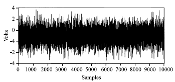
Fig. 2:	Input Gaussian noise

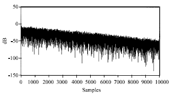
Fig. 3:	Residual noise of LMS algorithm

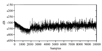
Fig. 4:	Residual noise of RLS algorithm

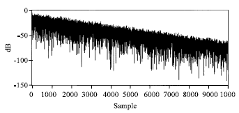Fig. 5:	Residual noise of Delta rule algorithm

The length of w(n) is chosen to be 96. The logistic function is used for the simulation of delta rule algorithm. All the weights are initialized to zero and all the results are average of 100 cycles.

All the simulations were done using MATLAB 6.5 (Release 12.1). The input white Gaussian noise of zero mean and unit variance is shown in the Fig. 2. The residual noise of LMS algorithm is shown in the Fig. 3. The residual noise of RLS and Delta rule algorithm is shown in the Fig. 4 and 5, respectively. RLS algorithm converges very quickly than the other two algorithms and the residual noise is also less. From the Fig. 4, the residual noise of Delta rule algorithm is less than the residual of LMS algorithm.

REFERENCES

- Douglas, S. and W. Pan, 1995. Exact expectation analysis of the LMS adaptive filter. IEEE Trans. Signal Process., 43: 2863-2871.
Direct Link - Glentis, G.O. K. Berberidis and S. Theodoridis, 1999. Efficient least squares adaptive algorithms for FIR transversal filtering. IEEE Signal Process. Maga., 16: 13-41.
Direct Link - Haykin, S., 1996. Adaptive Filter Theory. 3rd Edn., Prentice Hall, New Jersey, ISBN: 0-13-322760-X.
Direct Link - Maeda, Y. and R.J.P. de Figueiredo, 1997. Learning rules for neuro-controller via simultaneous perturbation. IEEE Trans. Neural Network, 8: 1119-1130.
Direct Link - Woo, T.K., 2001. Fast hierarchical least mean square algorithm. IEEE Signal Process. Lett., 8: 289-291.
Direct Link
k.vIJAYALAKSHMI Reply
Dear Sir, This is very extra ordinary paper and Good research work done by scholar.Excellent.
K.Mohanasundram Reply
Dear Sir,
I referred 5 times in this journal very extra ordinary technical work done by scholar.Surely this is very helpful for all the research scholars.
Dr K.Suresh Kumar Reply
This paper is very helpful for my entire Phd work and thesis .Kindly publish papers more and more then only very helpful for lot of scholars.