ABSTRACT
A new procedure based on conjugate gradient projection method for solving linear programming problems is given. This procedure presented here consists of a sequence of moves in the interior of the polyhedron set representing the feasible region until the optimal point is reached in at most m+n steps. Sensitivity analysis when changes in the objective function coefficients are occurred is investigated. The task of this analysis is to find the range of parameter to maintain the optimality for the given optimal point under the effect of these changes A simple production example is given to clarify the theory of the given procedure.
PDF Abstract XML References Citation
How to cite this article
URL: https://scialert.net/abstract/?doi=tasr.2019.7.11
INTRODUCTION
The problem of linear programming (LP) is one of the earliest formulated problems in mathematical programming, where a linear function has to be maximized (or minimized) over a convex constraint polyhedron X. This kind of problem has been widely applied in practically every area of production, economic, social and government planning.
The simplex algorithm was early suggested for solving this problem by moving toward a solution on the exterior of the constraint polyhedron X. In 1984, the area of linear programming underwent a considerable change of orientation when Karmarkar1 introduced an algorithm for solving (LP) problems which moves through the interior of the polyhedron. The algorithm of Karmarkar's and subsequent additional variants2,3 established a new class of algorithms for solving linear programming problems known as the interior point methods .While methods based on vertex information may have difficulties as problem's size increases, the interior point methods proved to be less sensitive to problem's size. For more details about interior point methods, the reader is referred to Ye4. Also for more recent work concerning interior point solution and conjugate gradient projection method, the reader is recommended to review5-8. Some time, it is quite important to know the range of parameters for which the solution remains optimal. The investigation that deals with changes in the optimal solution due to changes in the data of the linear programming problems can be found in Arsham9, Ghaffari-Hadigheh et al.10 and Hadigheh et al.11. In this study, an iterative method for solving (LP) problems with sensitivity analysis is given. This analysis presented here permits perturbation in the data of the objective function that maintain the optimality of the problem.
PROBLEM STATEMENT AND THE SOLUTION CONCEPT
The linear programming problem (LP) arises when a linear function is to be maximized over a convex constraint polyhedron X. This problem can be formulated as follows:
| (1) |
where, p, x∈Rn, A is an (m+n)×n matrix, b∈Rm+n, it pointed out that the nonnegative conditions are included in the set of constraints. This problem can also be written in the form:
 | (2) |
where, ![]() represents the ith row of the given matrix A, then it has in the non-degenerate case an extreme point (vertex) of X lies on some n linearly independent subset of X. It shall give an iterative method for solving this problem, this method starts with an initial feasible point then a sequence of feasible directions toward optimality is generated to find the optimal extreme point of this programming, in general if xk-1 is a feasible point obtained at iteration k-1 (k = 1, 2...) then at iteration k our procedure finds a new feasible point xk given by:
represents the ith row of the given matrix A, then it has in the non-degenerate case an extreme point (vertex) of X lies on some n linearly independent subset of X. It shall give an iterative method for solving this problem, this method starts with an initial feasible point then a sequence of feasible directions toward optimality is generated to find the optimal extreme point of this programming, in general if xk-1 is a feasible point obtained at iteration k-1 (k = 1, 2...) then at iteration k our procedure finds a new feasible point xk given by:
| (3) |
where, dk-1 is the direction vector along which it move and given by:
| (4) |
where, Hk-1 is an n×n symmetric matrix given by:
| (5) |
In Eq. 5, I is an n×n identity matrix and q is the number of active constraints at the current point while ![]() is defined as follows, for each active constraint s; s = 1, 2... q:
is defined as follows, for each active constraint s; s = 1, 2... q:
| (6) |
With, H0k-1 = I. Then Hk-1 is given by Hk-1 = Hqk-1. The step length αk-1 is given by:
| (7) |
The above relation stated that αk-1 is always positive. Proposition 2-3 shows that such a positive value must exist if a feasible point exists. Also due to the well known Kuhn-Tucker condition12,6 for the point xk to be an optimal solution of the linear program (2-1) their must exist u>0 such that:
| (8) |
where, Ar is an nxn sub-matrix of the given matrix A containing only the coefficients of the set of active constraints at the current point xk. This fact will act as a stopping rule of our proposed algorithm.
A NEW ALGORITHM FOR SOLVING (LP) PROBLEMS
The algorithm presented on this section for solving (LP) problems consists of the following steps:
| Step 0: | Set k=1, Ho =I, d0 =p, let x0 be an initial feasible point and apply relations (Eq. 7) to compute α0 |
| Step 1: | Apply relation (Eq. 3) to find a new solution xk |
| Step 2: | Apply relation (Eq. 8) to compute u, if u>0 stop. The current solution xk is the optimal solution otherwise go to step 3 |
| Step 3: | Set k = k+1, apply relations Eq. 5, 4 and 7 to compute Hk-1, dk-1 and αk-1, respectively and go to step 1 |
Remark 3-1: Assuming that q is the number of active constraints at point xk then if q<n and relation (Eq. 8) is satisfied this indicates that xk is an optimal non-extreme point, in this case the objective function can not be improved through any feasible direction and then we have Hk p = 0 at this point xk, it noted that although the matrix Hk is singular it does not cause the breakdown of this algorithm but indicate that all subsequent search directions dk+1 will be orthogonal to p.
Remark 3-2: If xk-1 is an extreme non-optimal i.e., there are n active constrains at point xk-1 and relation Eq. 8 is not satisfied.
A sub-matrix from the given matrix Ar is chosen (at least one constraint has to be dropped) to define a direction dk-1 for the new movement. This sub-matrix is normal to a column (aw) from (Ar)–1 such that pT (aw) is the most negative element in Eq. 8.
Theorem 3-1: Our procedure solves the (LP) problem in at most m+n iterations.
Proof: Since in each iteration it added at least one active constraint, then the optimal point may be reached in n steps and the algorithm terminate in at most n iterations. On the other hand if at any iteration we have non optimal extreme point and at least one constraint has to be dropped from the set of active constraints. Since our allowed directions by (Eq. 4) that improve the value of the objective function lies in the nullity of a subset of the constraint set, then it is moving in the direction parallel to a certain subset of the (m+n) constraints and hence in the worst case the maximum number of iterations required to reach the optimal point is limited by m+n.
SENSITIVITY ANALYSIS FOR LINEAR PROGRAMMING PROBLEM
Introducing a scalar parameter in the objective function coefficient of (LP) problem may affect the optimal solution due to some changes on the data of the objective function.
Now consider the perturbed (LP) problem when changes in the coefficient of the objective function is occurred and is formulated as:
 | (9) |
where, μ is a scalar parameter and p1∈Rn. Our task of this sensitivity analysis is to find the range of μ that maintain the optimality of the linear programming problem using the same argument then the only change will be in computing:
| (10) |
and for the optimal point to remain optimal u (μ )>0 has to be satisfied which gives the range of μ for the optimal point to remain optimal for the new perturbed problem (Eq. 9).
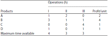
An application to production example: A small company manufactures four types of products. The data summarized the production hours per unit in each of three production operations and the profit per each unit is also given:

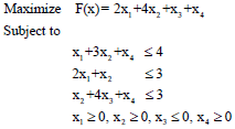
Assuming that the company wants to maximize profit, how many units of each product should be manufactured . For example suppose that x1, x2, x3 and x4 represent the number of units for each product, respectively, the above problem can be formulated as a linear programming problem:

| Step 0: |  |
| then Eq. 7 gives α0 = 0.1 and we go to step 1 | |
| Step 1: | Apply relation (Eq. 3) to get: |
 | |
| Step 2: | For this point x1 the first constraint is the only active constraint and since relation (Eq. 8) is not satisfied indicates this point is not optimal |
| Step 3: | Set k = 2. Apply relation (Eq. 5, 4 and 7) to get: |
 |
| Step 1: | Apply relation (3) to get: |
 | |
| Step 2: | For this point x2 the first and the third constraint are the only active constraints and since relation (8) is not satisfied |
| Step 3: | Set k = 3. Apply relation (Eq. 5, 4 and 7) to get: |
 |
| Step 1: | Apply relation (Eq. 3) to get: |
 | |
| Step 2: | For this point x3, it has the first, the second and the third constraint are the active constraints, since relation (Eq. 8) is not satisfied we go to step 3 |
| Step 3: | Set k = 4. Apply relation (Eq. 5, 4 and 7) to get: |
 | |
| we use relation (3) to get: | |
 |
Since relation (Eq. 8) is satisfied with uT = 1.1 0.45 0.25 0.35 this indicates that the extreme point x4 is the optimal point for the above linear programming problem with optimal value F(x4) = 6.5.
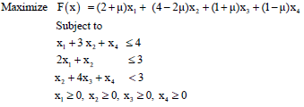
Sensitivity analysis has to be done if the given problem to be solved is taken the form:

Since for μ = 0, it has the extreme point x4 is the optimal point and relation (Eq. 8) is satisfied with uT = 1.1 0.45 0.25 0.35, then for the perturbed problem when a scaler parameter μ is added in the objective function we have to apply (Eq. 10) to compute:
uT(μ) = (1.1-0.9 μ 0.45+0.95 μ 0.25-0.25 μ 1.35-4.15 μ)
which gives the range of μ:
-0.47<μ<0.33
as the range such that the optimal extreme point x4 remains optimal for the perturbed problem.
CONCLUSION
In this study, it gave an iterative procedure for solving the linear programming problems with inequality constraints. The procedure is based on moving in the interior of the polyhedron through a sequence of feasible directions toward optimality. This procedure is used to study the effect for some change of the data of the objective function on the optimal solution of the given problem . Also the given method can be applied to other mathematical programming problems such as the linear fractional programming problem.
SIGNIFICANCE STATEMENT
This study discovered a new procedure for solving the linear programming problem that can be beneficial for some sensitivity investigation concerning the optimality of the given problem and this study will help the researchers to uncover the critical areas of many optimization problems that many researchers were not able to explore. Thus a new theory on classical sensitivity analysis for mathematical programming problems may be arrived
REFERENCES
- Karmarkar, N., 1984. A new polynomial-time algorithm for linear programming. Combinatorica, 4: 373-395.
CrossRefDirect Link - Adler, I., M.G. Resende, G. Veiga and N. Karmarkar, 1989. An implementation of Karmarkar's algorithm for linear programming. Math. Program., 44: 297-335.
CrossRefDirect Link - Vanderbei, R.J., M.S. Meketon and B.A. Freedman, 1986. A modification of Karmarkar's linear programming algorithm. Algorithmica, 1: 395-407.
CrossRefDirect Link - Goldfarb, D. and L. Lapidus, 1968. Conjugate gradient method for nonlinear programming problems with linear constraints. Ind. Eng. Chem. Fundamen., 7: 142-151.
CrossRefDirect Link - Sun, Q. and Q. Liu, 2006. Global convergence of modified hs conjugate gradient method. J. Applied Math. Comput., 22: 289-297.
CrossRefDirect Link - Wang, W., 2002. The convergence of an interior-point method using modified search directions in final iterations. Comput. Math. Applic., 44: 347-356.
CrossRefDirect Link - Arsham, H., 2007. Construction of the largest sensitivity region for general linear programs. Applied Math. Comput., 189: 1435-1447.
CrossRefDirect Link - Ghaffari-Hadigheh, A., H. Ghaffari-Hadigheh and T. Terlaky, 2008. Bi-parametric optimal partition invariancy sensitivity analysis in linear optimization. Central Eur. J. Operat. Res., 16: 215-238.
CrossRefDirect Link - Hadigheh, A.G., K. Mirnia and T. Terlaky, 2007. Active constraint set invariancy sensitivity analysis in linear optimization. J. Optim. Theor. Applic., 133: 303-315.
CrossRefDirect Link


