
A. Eide
Norwegian College of Fishery Science, University of Troms�, Norway
A. Wikan
Harstad University College, Norway
Journal of Fisheries and Aquatic Science
Year: 2010 | Volume: 5 | Issue: 6 | Page No.: 454-468


ABSTRACT
We explore a fishery targeting the mature part of a stock, while by catching the immature part. Both targeted catch and bycatch may have positive market values. Cost of effort is supposed to be a function of the selection properties of the fishing gears. Mature fish is assumed to cannibalise on the immature part of the stock. A bioeconomic model of the problem is set up and it is shown that the model possesses a unique nontrivial stable equilibrium and moreover that both cannibalism and catch act as stabilising factors. Necessary conditions for a bioeconomic optimum are also provided. The model is applied on the Northeast Arctic cod stock where time series of stock biomasses, catches and fishing mortality rates covering the period 1946-2000 have been used to estimate the model parameter values. The economic parameters have been estimated on the basis of previous open access to the fishery, assuming bioeconomic equilibrium. It is shown that bioeconomic optimum could not be obtained at any discount rate, without reducing the rate of fishing mortality, first of all on the mature part of the cod population.
PDF Abstract XML References Citation
Received: December 02, 2009;
Accepted: April 06, 2010;
Published: May 29, 2010
How to cite this article
A. Eide and A. Wikan, 2010. Optimal Selection and Effort in a Fishery on a Stock with Cannibalistic Behaviour the Case of the Northeast Arctic Cod Fisheries. Journal of Fisheries and Aquatic Science, 5: 454-468.
DOI: 10.3923/jfas.2010.454.468
URL: https://scialert.net/abstract/?doi=jfas.2010.454.468
DOI: 10.3923/jfas.2010.454.468
URL: https://scialert.net/abstract/?doi=jfas.2010.454.468
INTRODUCTION
As documented by Myers et al. (1990) several commercially important fish stocks exhibit significant year by year biomass fluctuations. The Northeast Arctic cod stock is one of these stocks and there is a lot of evidence of such behaviour in the past, also before the development of industrial cod fisheries (Hjort, 1914; Qiestad, 1994). Long time observed catch fluctuations and cod stock estimates from 1946 to 2000 indicate a close connection between biomass fluctuation and age composition within the stock (Anonymous, 2001).
In most periods strong year-classes seem to dominate the stock, while a more harmonised year-class composition occurs in other periods. Shifts in year-class composition seem to influence the stock fluctuation in biomass and the variations are not necessarily reflecting variations in individual growth parameters. Another possible explanation is that the cod stock avoids or minimises the effect of changes in individual growth through cannibalistic behaviour and indeed, the cannibalistic behaviour of cod has been verified through stomach analysis (Bogstad et al., 1994).
This has important dynamical consequences. We have earlier shown that in the interplay between increasing fecundity and increasing cannibalism pressure, the former turns out to be a destabilising effect whiles the latter tends to stabilise (Wikan and Eide, 2004). Predation on the stock by other species may also stabilise the dynamics, but there are important cases where predation and cannibalism act differently (Wikan, 2001). Other examples of dynamical consequences of cannibalism may be found in Gurtin and Levine (1982), Cushing (1991), Van den Bosch and Gabriel (1997) and Magnússon (1999). Cushing (1991) describes the stabilising self-regulation property of cannibalism and Kohlmeier (1995) elaborates the stabilising role further also in a predator-prey context. The latter includes cannibalism in the net growth expressed by one differential equation covering a cannibalistic predator. There is also a vast literature on bioeconomic prey-predator models, reported by Hannesson (1983), Ragozin and Brown (1985), Wilen and Brown (1986), Flaaten (1991) and Brock and Xepapadeas (2004).
Unlike the research quoted above, the scope of this study is to identify social optimal equilibriums for the Northeast Arctic cod fishery by taking the cannibalistic behaviour of the stock into consideration. The biological model used is in principle a symbiotic model consisting of two differential equations which describe a cannibalistic relationship between mature and immature cod. Furthermore, a linear harvest equation and simple revenue and cost equations are applied. Biological and economic parameters are estimated from a time series covering the period 1946-2000.
Fleet dynamics are not included in the model presented, as the selective properties of fishing gears and fishing effort produced are considered being control variables and management means rather than a result of economic dynamics. This issue is later discussed in the case of unrestricted open access fisheries.
THE MODEL
Let x (t) and y (t) be the mature and the immature parts of a population at time t, respectively and assume further that the dynamics of x and y may be described by the nonlinear system
| (1) |
where,
 | (2) |
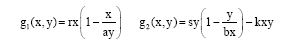
(1) may be regarded as a minor modification of the prey-predator model presented by May and co-workers (May et al., 1979), including a positive symbiotic relationship in the prey-predator interaction. The constants a, b, r, s and k are all assumed to be positive. r and s are the intrinsic growth rates of the mature and immature part of the population, respectively. The relation ![]() expresses that the natural equilibrium level of the mature stock is directly related to the abundance of immature by the proportionality factor a. Similarly
expresses that the natural equilibrium level of the mature stock is directly related to the abundance of immature by the proportionality factor a. Similarly ![]() expresses that the natural equilibrium level of the immature stock relates to the mature stock by the proportionally factor b. The relationships expressed by a and b cover the non-cannibalistic net growth interaction, including the recruitment of surviving immature to the mature fraction of the stock and the recruitment of immature as a function of the spawning biomass. Cushing (1991) points out the double effect cannibalism has on the adult (mature); both by affecting immature survival to become mature and providing the mature with an additional source of energy.
expresses that the natural equilibrium level of the immature stock relates to the mature stock by the proportionally factor b. The relationships expressed by a and b cover the non-cannibalistic net growth interaction, including the recruitment of surviving immature to the mature fraction of the stock and the recruitment of immature as a function of the spawning biomass. Cushing (1991) points out the double effect cannibalism has on the adult (mature); both by affecting immature survival to become mature and providing the mature with an additional source of energy. ![]() contains a somewhat crude form of cannibalism relation, assuming the immature part of the population to be consumed at a rate proportional to their density per mature biomass. k will be referred to as the cannibalism parameter. The overall effect on the immature may be more easily seen when g2 (x, y) is reformulated to
contains a somewhat crude form of cannibalism relation, assuming the immature part of the population to be consumed at a rate proportional to their density per mature biomass. k will be referred to as the cannibalism parameter. The overall effect on the immature may be more easily seen when g2 (x, y) is reformulated to
where, the expression (s-kx) corresponds to the intrinsic growth rate of a logistic growth equation and bx (s-kx)/s the equilibrium biomass. Both are functions of the mature stock, the intrinsic growth rate being reduced by cannibalism (represented by the parameter k), while two mechanisms affect the equilibrium biomass, the recruitment (represented by the parameter b) and cannibalism.
The model was initially proposed by Eide (1987) and has later been applied in several bioeconomic studies where cannibalism plays an important role (Armstrong, 1999; Armstrong and Sumaila 2000, 2001).
Let us now extend model Eq. 1 by including catch. Assume that x is the target of harvest with a bycatch of y, depending on the selection properties of the fishing gears. The selection parameter isα, α≥0. The special case α = 0 gives no bycatch of y, while α = 1 represents the situation of no selection and consequently equal fishing mortalities f for x and y. Hence, the annual harvest of the targeted mature part of the stock, h1 and the bycatch, h2, are described by
| (3) |
Including harvest the model is expressed by
| (4) |
The unique nontrivial equilibrium of (4) is found to be
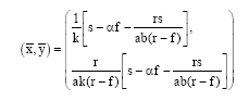 | (5) |
where, s>αf, r>f and s-αf>rs [ab (r-f)]-1 are necessary constraints in order to ensure biological acceptable equilibrium (non-negative biomasses). Denoting the Jacobian of (4), evaluated at equilibrium by J, the trace (tr) and determinant (det) of J are
| (6a) |
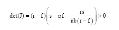 | (6b) |
Hence, the equilibrium ![]() is locally stable. From a dynamic point of view this finding allow us to conclude that increased harvest may not give birth to nonstationary behaviour, a result which to a great extent is in accordance with the findings of Wikan and Eide (2004).
is locally stable. From a dynamic point of view this finding allow us to conclude that increased harvest may not give birth to nonstationary behaviour, a result which to a great extent is in accordance with the findings of Wikan and Eide (2004).
In the next section we assume x and y to represent the mature and the immature fractions of the Northeast Arctic cod stock respectively. Catch data and stock biomasses from the period 1946-2000 are employed in order to estimate the model parameters r, s, a, b and k in (1), (2).
BIOLOGICAL GROWTH PARAMETER ESTIMATES
As the data set presented in Table 1 is a discrete time representation of the dynamic system, (1), (2) has to be rewritten as discrete time equations in order to estimate parameter values of the five a priori positive parameters (a, b, r, s and k). Total annual growth of the mature and immature fraction (corresponding to differential Eq. 2) may then be expressed as:
| (7) |
and
| (8) |
Mature and immature biomasses of year t+1 (including the error term u) are obtained from the data set of year t, assuming the discrete version of model (6). The model’s biomass estimates at given parameter values are denoted ![]() and
and ![]() .
.
| (9) |
and
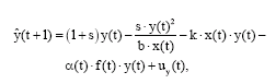 | (10) |
for t∈[1946, 2000].
It should however be noted that the biomasses in Table 1 in this study are treated as data even though they really are estimates calculated on the basis of catch data and an accounting method known as Virtual Population Analysis (VPA, or XSA which is the extended version also including additional features to utilise other information through tuning methodology Anonymous (2001). In this study the XSA estimation method is regarded as a measuring method rather than model estimates, as the stock biomasses are measured through methodology build on relative consistency within year classes. Uncertainties regarding actual biomass level are real, but not relevant for our model, as biomass indexes, not necessarily real values, are sufficient to parameterise the model.
As in Wikan and Eide (2004) system parameters are estimated simultaneously by identifying parameter sets of local minimums of the squared sum of total (mature and immature) biomass.
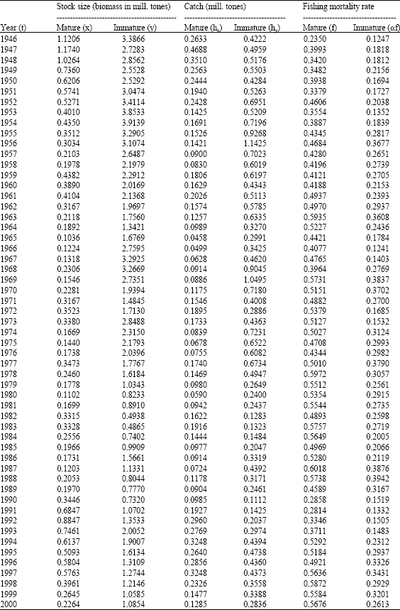
| Table 1: | The Northeast Arctic cod stock biomass and catches in million tons 1946-2000. The figures are from ICES’ Advisory Committee on Fisheries Management (Anonymous, 2001) tables 3.7 (catches), 3.19 (stock biomass) and 3.23 (maturity) |
 | |
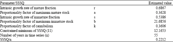
| Table 2: | Estimated parameters of Eq. 2 found by minimising (11), applying data of Table 1 |
 | |
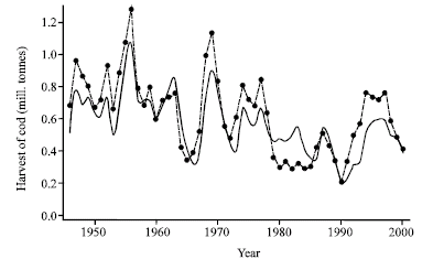 | |
| Fig. 1: | Estimated total catch of mature and immature cod 1946-2000 by use of (1), (2) and (6). Initial stock sizes are taken from 1946 and historical fishing mortalities (Table 1) have been used. The points connected by the dashed curve represent actual annual historical catches (Table 1) over the same period |
 | (11) |
While only accepting non-negative parameter values. The best fit parameter set is presented in Table 2 and shown in Fig. 1. Eide (1987) employs a weighted sum of squared residuals in the mature and immature biomasses instead of the flat sum in Eq. 11. Separating into mature and immature fractions may however become a critical factor in the estimation process and since this separation is uncertain (in particular for the first part of the time series; Anonymous, 2001), a method focusing total biomass rather that the biomass fractions of immature and mature biomasses, was preferred in this study.
The estimation was carried out by numerical methods searching for a regional minimum of (11) within valid parameter space. A program based on internal minimizing function in the software Mathematica© was used in the numerical estimation procedure. The algorithms and Mathematica© notebook used for parameter estimations may be obtained by contacting the corresponding author.
As shown in Fig. 1 the model has an acceptable fit to historical data, indicating that a large part of the observed fluctuations may be explained by the model. The model phase plot in absence of fishery Fig. 2 shows natural equilibrium as a stable focus close to the initial stock situation in 1946.
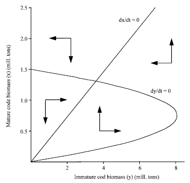 | |
| Fig. 2: | Phase plot of the natural growth system (1) and (2), parameter values from Table 2. Note that the displayed system does not include fishing mortalities as fleet dynamics is not included |
HARVEST ECONOMY MODEL AND PARAMETER ESTIMATES
Now turn to the economic aspects of fishing. A simple economic model is set up and parameterised assuming essentially an open access fishery in the past. Available variables for managing the fishery are gear selection and any measures controlling total fishing effort.
Denoting constant unit prices on catch from the two fractions (x and y) for p1 and p2, respectively, total annual revenue (TR) of the fishery may be expressed as:
| (12) |
or equivalently, by use of the definitions of h1 and h2 (cf. (5)) as:
| (13) |
The Total Cost (TC) simply reflects the cost of producing a certain amount of fishing mortality. Assuming a constant unit cost of fishing effort and a linear relationship between rate of fishing mortality and fishing effort, there will be a constant unit cost of fishing mortality rate. Fishing effort is the fishing activity produced by labour (fisher) and capital (boat and fishing gear) and the unit cost of effort includes the opportunity costs of these input factors, by which a normal profit is obtained when total revenue covers the total costs. In this case the possibility of a selective fishery is included, so the basic assumption of constant unit cost of effort is related to a given, fixed selection property of the fishing fleet.
Let c1 be the unit cost of fishing effort in the case of no selection (selection value α = 1). Assume further that selective fishery (α≠1) involves a larger unit cost of fishing effort, as selection is obtained by making the fishing gears less efficient in fishing immature cod (α<1) or more efficient in fishing mature cod (α> 1). Specifically targeting mature or immature fish therefore involves costs both by reducing the probability of fishing the non-targeted part and by increasing the probability of fishing the targeted. The former is obtained by technologically changing the gear (essentially making it less efficient), while the latter is obtained by technological changes increasing the probability of catching the target mature fraction of the stock.
Change in unit cost of fishing mortality is given by c2. Total cost (including all opportunity costs) will be a function of f and α with a minimum when α =1. Further
whenever α≥0. Throughout the paper the following cost function is assumed,
| (14) |
which is consistent with the given constraints, where c1and c2 are constant cost parameters (c1≥0, c2≥0). Note that TC increases as α is increased or decreased from the non-selective value 1.
Resource rent obtained from the fishery, π, is the a function of stock size (x) and effort (here given by the fishing mortality rate f),
| (15) |
It is well known that bioeconomic equilibrium of a fishery of one control variable (fishing effort)-if existing-is defined by
 | (16) |
The TR and TC refer to equations (13) and (14). The individual decision maker may be controlled by the selection value (α) and the fishing mortality rate (f) in the fishery. According to Eq. 14 the unit cost of effort has its minimum when α =1, which will be the open access selection value when no capacity constraints and technological regulations are put on the harvesting units.
Equality (16) should therefore be a valid criterion of open access or bioeconomic equilibrium also in this case. Inserting (14) and (15) and substituting x and y by applying the nontrivial equilibrium (7) the bioeconomic equilibrium criterion (16) (when α = 1) is
| (17) |
(17) is a cubic function of f, by which one root will be the bioeconomic equilibrium solution if an open access solution exists.
Generally, mature cod is regarded as a more valuable product than the immature. In this analysis prices are assumed to be 12 and 8 NOK per kilo respectively for mature and immature cod, while the cost parameters have been estimated on the basis of assumed prices and the basic assumption of normal profits in the fishery, from the data of Table 1 and profit Eq. 15.
| Table 3: | Assumed price parameter values and estimated cost parameter values when c2 = 2 c1. The cost parameter estimation was done by minimising*. All values are measured in Norwegian currency, NOK |
 | |
 | |
| Fig. 3: | Cost Eq. 14 as a function of fishing mortality rates (f) and selection values (α) |
The estimation of cost parameters is based on assuming zero average resource rent during the period, which seems reasonable even after introducing catch restrictions.
Since no available information was found on the cost of selection, unit cost of effort in case of 100% catch selectivity (no immature catch, α = 0) is assumed to be twice the unit cost of no selection, e.g., c2 = 2.c1. The economic parameter values obtained on the basis of these assumptions are presented in Table 3 and Fig. 3.
When assuming a constant discount rate δ, present value of the resource rent from the fishery over all time is
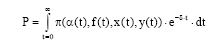 | (18) |
Our next goal is to maximise (18) subject to (4) where x(t) and y(t) are regarded as state variables and α (t) ε [0, ∞], f (t) ε[0, ∞] are the controls. By use of the current value formulation, the Hamiltonian of the problem is
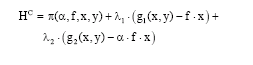 | (19) |
where, λi = λi (t), i = 1, 2 are the adjoint functions. Further, from the maximum principle
| (20) |
The subscripts x and y denote the derivatives with respect to x and y. If we additionally suppose optimal controls to be located in the interior of the convex control region, we have:
| (21) |
Finally, using the fact that the bioeconomic model (4) possesses a unique nontrivial stable equilibrium (5), we find after some algebra from (20) and (21) that the optimal controls α* and f* (at equilibrium) may be obtained from the relations
 | (22a) |
 | (22b) |
where, x, y, π,…. must be evaluated at equilibrium. Note that (22a, b) are cubic equations in α* and f* and must be solved by means of numerical methods.
RESULTS AND DISCUSSION
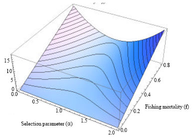
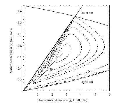
Numerical solutions α* and f* of (22a, b) for different values of the discount rate δ are shown in Table 4, where estimated values of r, a, s, b and k from Table 2 and estimated prices and cost parameters p1, p2 c1 and c2 from Table 3, have been applied. The numerical solutions are also shown together with a contour plot of total profit in Fig. 4, as a curve connecting different f-α combinations of maximum profit for varying values of the discount rate δ.
As pointed out in the previous part, a selection parameter α =1 (no selection) is assumed in the case of open access, since possible benefits of choosing α>1 partly will be future benefits, while α<1 both causes higher cost and less catch.
| Table 4: | Bioeconomic equilibrium (open access solution constrained by α = 1), Eq. 17 and optimal conditions (22a, b) for different values of the discount rate as illustrated in Fig. 4. Current state (year 2000) and average values for the period 1946-2000, with resource rent calculation equal annual average, are also provided. x and y in million tons. The π (annual resource rent from Eq. 15, while including opportunity cost of labour and capital) in billion NOK. |
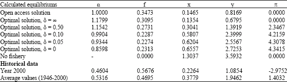 | |
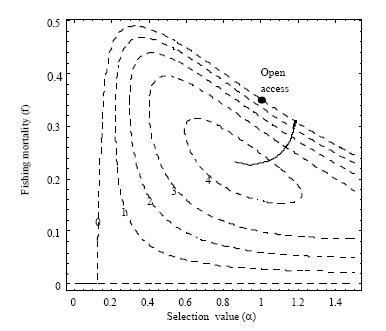 | |
| Fig. 4: | The dashed curves represent isovalues (of 0, 1, 2, 3 and 4 billion NOK, respectively) of total resource rent of the fishery (Eq. 15), while the solid line gives the unique solution of the two optimal equilibrium conditions (22a, b) for non-negative values of the discount rate (δ), starting at the maximum resource rent location when δ = 0, all as functions of the system control variables α and f. The point indicates bioeconomic equilibrium constrained by α = 1 (Eq. 17) |
There may however be reasons for the fleet to increase the selection value, making the a priori assumption less reliable. Since the optimal equilibrium solution of δ = ∞ (Table 4 and in Fig. 4, 5) is found at a selection value about 18% higher than one, the a priori condition of α = 1 may not hold for an unrestricted open access fishery.
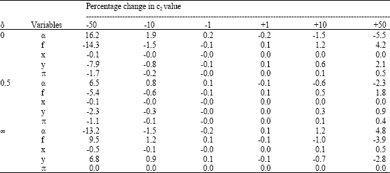
As a high degree of uncertainty is related to the values of the parameters in the cost equation, a sensitivity analysis on the effect of changes in the value of c2 was performed and the results are displayed in Table 5.
Historical fluctuations in the Northeast Arctic Cod fishery are reasonably well explained by the simple cannibalistic model presented in this paper and the year to year variation in fishing effort. The symbiosis or cannibalism model (1), (2) describes coexistence of the immature and mature fractions of a population, both benefiting and depending of each other, at the same time as immature are preyed upon by the mature fraction. The five model parameters, whereby one (k) expresses the cannibalistic relationship, are lumped based parameters covering a range of different biological processes. Two parameters (a and b) are closely linked to recruitment relationships between the two fractions, maturation and, indirectly, therefore also to cannibalism. The intrinsic growth rates (r and s) also are lumped based parameters; covering individual growth, density dependency, mortalities, etc.
The economic model summed up by the resource rent Eq. 15 is similarly simple, including a cost of selective harvesting. This particular cost is believed to increase both when increasing efficiency in catching mature fish or reducing efficiency in catching immature fish. When reducing the catch of immature fish, a minimum is reach when no immature fish catch is obtained at α = 0. As there is no theoretical constraints on increasing efficiency in catching mature fish, there is no corresponding value limiting α upwards, making it perfectly possible to have α-values larger than 1.
 | |
| Fig. 5: | Phase plot of the system state variables x and y (solid lines, see also Fig. 2) and contour plot of Eq. 15 at equilibrium (dashed curves) showing isocurves of -10, -5, 0, 1, 2, 3 and 4 billion NOK, as indicated. As in Fig. 4 the calculated optimal points of different discount rates are represented as a solid line drawn from the maximum point, ending close the constrained bioeconomic equilibrium of α = 1 (filled circle point) when δ = ∞. Average combined biomasses over the period 1946-2000 (from Table 4) are shown as an asterisk surrounded by a circle |
| Table 5: | Sensitivity analysis on the impact choice of parameter value of c2 has on the two control variables α and f and the state variables x and y. All values in percentage change from three of the basic runs in Table 4, namely the α-values 0, 0.05 and infinity |
 | |
Also note that investments in selective fishery by avoiding catching immature fish, over time also increases the available mature part of the stock, as more immature fish survive this period.
The Northeast Arctic Cod fishery is a fishery where it has been put a lot of effort into protecting juveniles and other immature cod from being caught. Consequently the α-value is expected to be significantly less than one. It should however be noted that the management objectives may not be the only explanation of the historical record shown in Table 4, as the relative density of mature fish is higher on the spawning grounds where a large share of the fish is caught (Anonymous, 2001). This may question if the cost equations employed here should have its lowest unit cost at a value closer to the historical average rather than at α = 1.
The results in Table 4 show how the social optimal α-value varies with the social discount rate δ. No selection, or rather negative selection (α-values higher than 1), is optimal at discount rates above 10%, while a perfectly selective fishery (α= 0) is never found to be optimal at any discount rate. The latter also turns out to be valid in the special case of c2 = 0 (no cost of selection). Equilibriums by other values of c2 have been studied in a sensitivity analysis (Table 5), indicating the same threshold value close to a discount rate of 10% where the optimal selection is no selection (α = 1). Reduced selection cost below a discount rate of 10% gives increased selection and reduced fishing effort in optimum equilibrium solution. The selection cost parameter does however not alter the general conclusions as these seem to be rather robust towards such changes.
In this study a constrained open access equilibrium is considered, a priori assuming a non-selective fishery (α = 1). The catch history and fishing on spawning grounds indicate however that the α-value in open access equilibrium more probably will be found between 0.5 and 1.0 and may even be below the α-value of maximum sustainable economic yield, which is 0.86 (at δ = 0 in Table 4). This may indicate that the historical open access equilibrium may be found even further from the optimal solution of δ = ∞ (Table 4) than the assumed open access presented here indicates. This may give reason to question if investments in mesh size regulations on nets and trawls and minimum size regulation on fish caught is inconsistent with a objective of social optimal regulation from a capital theoretic point of view.
As seen in Fig. 6b the selection factor (α) in the period 1946-2000 varied between 0.3- 0.6 with a mean value of α = 0.5316 (Table 4). Mesh size regulation was first introduced in the 1960s, but low selection values, at least in the early years, reflect the fishing pattern referred to above; the winter-spring fishery on the coastal spawning grounds being the most important. Juveniles of the migrating cod stock are available in the open sea fisheries, mainly exploited by trawlers. Since today’s selection factor is far below calculated optimal values of any level of discount rates, it may be argued that relatively the open sea fishery should increase their share in order to obtain optimal exploitation. Less surprising, Table 4 also confirms that current fishing mortality rate on mature cod is much higher than what is found to be the social optimal fishing mortality rate (at equilibrium), independent on discount rate value. At a discount rate of 5%, optimal fishing mortality rate of mature cod is close to the fishing mortality rate of immature cod in year 2000 (αf), which actually is close to the optimal equilibrium value, as this optimum in practical terms is a non-selective fishery.
How far the actual fishery has been from an equilibrium situation is indicated by the two panels in Fig. 6, both showing equilibrium iso-resource rents as functions of combinations of stock biomasses (Fig. 6a) and combinations of selection and fishing mortality rates (Fig. 6b). In the first case the changes in stock sizes pass through the area of maximum resource rent before settling down at a lower stock size area. Figure 6b shows however, that the maximum resource rent in equilibrium is far from the historical values of the selection parameter and fishing mortality rates over the period.
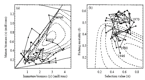 | |
| Fig. 6: | Historical data 1946-2000 from Table 1 (solid lines) placed in the phase plot of the system from Fig. 2 and 5 (left) and the contour plot from Fig. 4 (right). The dashed isocurves indicate resource rent equilibriums of 0, 1, 2, 3 and 4 billion NOK |
Based on these findings it is reasonable to assume a twofold management problem, aiming to maximise the present value of all future resource rent from the fishery; 1) Reducing the overall fishing mortality and 2) Changing the selection pattern towards a less selective fishery, relatively increasing the share placed on the immature fraction of the stock.
REFERENCES
- Armstrong, C.W. and U.R. Sumaila, 2000. Cannibalism and the optimal sharing of the Nort-East Atlantic cod stock: A bioeconomic model. J. Bioecon., 2: 99-115.
CrossRefDirect Link - Armstrong, C.W. and U.R. Sumaila, 2001. Optimal allocation of TAC and the implications of implementing an ITQ management system for the North-East Arctic cod. Land Econ., 77: 350-359.
Direct Link - Armstrong, C.W., 1999. Sharing a fish resource-Bioeconomic analysis of an applied allocation rule. Environ. Resour. Econ., 13: 75-94.
CrossRefDirect Link - Brock, B.W. and A. Xepapadeas, 2004. Management of interacting species: Regulation under nonlinearities and hysteresis. Resour. Energy Econ., 26: 137-156.
Direct Link - Flaaten, O., 1991. Bioeconomics of sustainable harvest of competing species. J. Environ. Econ. Manage., 20: 163-180.
CrossRef - Gurtin, M.E. and D.S. Levine, 1982. On populations that cannibalize their young. SIAM J. Applied Math., 42: 94-108.
Direct Link - Hannesson, R., 1983. Optimal harvesting of ecologically interdependent fish species. J. Environ. Econ. Manage., 10: 329-345.
Direct Link - Kohlmeier, E., 1995. The stabilizing role of cannibalism in a predator-prey system. Bull. Math. Biol., 57: 401-411.
CrossRefDirect Link - Magnusson, K., 1999. Destabilizing effect of cannibalism on a structured predator-prey system. Math. Biosci., 155: 61-75.
PubMed - May, R., J.R. Beddington, C.W. Clark, S.J. Holt and R.M. Laws, 1979. Management of multispecies fisheries. Science, 205: 267-277.
Direct Link - Qiestad, V., 1994. Historic changes in cod stocks and cod fisheries: Northeast Arctic cod. ICES Mar. Sci. Symp., 198: 17-30.
Direct Link - Ragozin, D.L. and G. Brown, 1985. Harvest policies and nonmarket valuation in a predator-prey system. J. Environ. Econ. Manage., 12: 155-168.
Direct Link - Van den Bosch, F. and W. Gabriel, 1997. Cannibalism in an age-structured predator-prey system. Bull. Math. Biol., 59: 551-567.
CrossRefDirect Link - Wikan, A. and A. Eide, 2004. An analysis of a nonlinear stage-structured cannibalism model with application to the North East Arctic cod stock. Bull. Math. Biol., 66: 1685-1704.
PubMedDirect Link - Wikan, A., 2001. From chaos to chaos. An analysis of a discrete age-structured prey-predator model. J. Math. Biol., 43: 471-500.
PubMed - Wilen, J. and G. Brown, 1986. Optimal recovery paths for perturbations of trophic level bioeconomic systems. J. Environ. Econ. Manage., 13: 225-234.
Direct Link