

A. Rajarathinam
Department of Statistics, Manonmaniam Sundaranar University, Tirunelveli-627 012, Tamil Nadu State, India
LiveDNA: 91.27341
P. Tamilselvan
Department of Statistics, Manonmaniam Sundaranar University, Tirunelveli-627 012, Tamil Nadu State, India
Journal of Applied Sciences
Year: 2021 | Volume: 21 | Issue: 1 | Page No.: 31-41





ABSTRACT
Background and Objective: The novel coronavirus pandemic, known as COVID-19, could not have been more predictable, thus, the world encountered health crises and substantial economic crises. This study analysed the trends in COVID-19 cases in October 2020 in four southern districts of Tamil Nadu state, India, using a panel regression model. Materials and Methods: Panel data on the number of COVID-19-infected cases were collected from daily bulletins, published by the Health & Family Welfare Department, Government of Tamil Nadu, India. Panel data regression models were employed to study the trends. EViews Ver.11. software was used to estimate the model and its parameters. Results: In all four districts, the COVID-19-infected case data followed a normal distribution. Maximum numbers of COVID-19-infected cases were registered in Kanyakumari, followed by Tirunelveli, Thoothukudi and Tenkasi districts. Very fewest COVID-19 cases were registered in Tenkasi, followed by Tirunelveli, Thoothukudi and Kanyakumari districts. A random-effects model was found to be an appropriate model to study the trend. Conclusion: The panel data regression model is found to be more appropriate than traditional models. The Hausman test and Wald test confirmed the selection of the random-effects model. The Jarque-Bera normality test ensured the normality of the residuals. In all four districts under study, the number of COVID-19 infections showed a decreasing trend at a rate of 1.68% during October, 2020.
PDF Abstract XML References Citation
Copyright: © 2021. This is an open access article distributed under the terms of the Creative Commons Attribution License , which permits unrestricted use, distribution and reproduction in any medium, provided the original author and source are credited.
How to cite this article
A. Rajarathinam and P. Tamilselvan, 2021. Estimating Trends in COVID-19 Infected Cases Based on Panel Data Regression Modelling. Journal of Applied Sciences, 21: 31-41.
DOI: 10.3923/jas.2021.31.41
URL: https://scialert.net/abstract/?doi=jas.2021.31.41
DOI: 10.3923/jas.2021.31.41
URL: https://scialert.net/abstract/?doi=jas.2021.31.41
INTRODUCTION
The 2019 COVID-19 pandemic has received much attention as it has affected most economies worldwide and resulted in innumerable deaths. Because no antiviral drugs or vaccines exist, the number of new coronavirus-affected cases has increased tremendously and many people have died. The development of various methodologies to analyse these pandemic data has become an especially important research area1.
An investigation has been made by estimating hidden models and trends of COVID-19 infected cases in all the 37 districts of Tamil Nadu State, India during the period from 1st August, 2020 to 31st December, 2020 by using different curve fitting tools. The result reported that decreases in trend have been observed in all the district1. Lockdowns and the effectiveness of reduction in the contacts in Italy have been measured using the modified model. The results showed a decrease in infected people due to stay-at-home orders and tracing quarantine interventions2. The prediction, regarding the number of COVID-19 cases in India based on a differential equation model. The model shows that the imposition of a countrywide lockdown plays an important role in restraining the spread of the disease3. A log-linear model has been used to estimate the progression of the COVID-19 infection in Tamil Nadu, India. The result indicates that the outbreak is showing decay in the number of infections of the disease which highlights the effectiveness of controlling measure4. Another study analyses the spatial distribution of COVID-19 incidence in Brazils municipalities (counties) and investigate its association with sociodemographic determinants to better understand the social context and the epidemic’s spread in the country using the Ordinary Least Squares (OLS), Spatial Autoregressive Model (SAR), Conditional Autoregressive Model (CAR) and the local regression model called Multiscale Geographically Weighted Regression (MGWR). The MGWR model fit improved when compared to the OLS, SAR and CAR5. A mathematical epidemic model is framed by taking inspiration from the classic Susceptible (S)-Infected (I)-Recovered (R), (SIR) model and develop a compartmental model with ten compartments to study coronavirus dynamics in India with the inclusion of factors related to face mask efficacy contact tracing and testing along with quarantine and isolation6. Autoregressive Integrated Moving Average (ARIMA) modelling approach has been used for projecting coronavirus (COVID-19) prevalence patterns in East African countries, mainly Ethiopia, Djibouti, Sudan and Somalia7. Dynamic Panel Data Modeling and Surveillance of COVID-19 in Metropolitan area in the United Stated using the longitudinal trend analysis and Wald test8.
In the ARIMA times series model the variable under study should be stationary. When the variable is not stationary one should convert the original data to the first or second difference. By making the original series into stationary series the estimated trend model is for the transformed series not for the original series. This is one of the main drawbacks of ARIMA time series modelling.
To avoid this problem, Panel Data Regression modelling can be used. By combining time series of cross-section observations, panel data give “more informative data, more variability, less collinearity among variables, more degrees of freedom with more efficiency”. As Baltagi9 stated that compared to pure cross-sectional and ARIMA time series, panel data regression estimation is better to identify and measure effects of independent variables on dependent variables, which one cannot measure using time series and cross-section data. The functional form of the equation, the slope coefficients, gives the percentage change in the dependent variable9.
Based on the above discussion the main purpose of the present study is to study the trends in the number of COVID-19 infected cases, i.e., whether the number of cases decreased or increased. Additionally, the impacts of COVID-19 in four different southern districts of Tamil Nadu, namely, Kanyakumari, Tenkasi, Thoothukudi and Tirunelveli (cross-sections), were investigated by using panel data models. These are the four districts that come under the Manonmaniam Sundaranar University, Tirunelveli, India. Based on the outcome of this study, the University authorities can take an appropriate academic decision whether to go for the online class, online examinations or offline class etc., based on the available COVID-19 infections trends in these four districts.
MATERIALS AND METHODS
Materials: The COVID-19 dataset was collected from the official Tamil Nadu Government website. In this novel study, only four southern districts of Tamil Nadu, including Kanyakumari, Tenkasi, Thoothukudi and Tirunelveli, were considered in October, 2020.
Methodology: Panel data are a type of data that contain observations of multiple phenomena collected over different periods for the same group of individuals, units or entities. In short, econometric panel data are multidimensional data collected over a given period. A simple panel data regression model is specified as9-11:
 | (1) |
where, νij is the estimated residuals from the panel regression analysis, Y is the dependent variable, X is the independent or explanatory variable, α and β is the intercept and slope, i is the ith cross-sectional unit, t is the tth month and X is assumed to be non-stochastic and the error term to follow classical assumptions, namely:
 |
In this study, i, the number of cross-sections is 4 (i = 1, 2, 3, 4) and t = 1, 2, 3…, 31.
Unit root test: Unit roots for the panel data can be tested using either the Leuin-Llin-Chu12 test or the Hadri13 LM stationary test. The null hypothesis is that panels contain unit-roots and the alternative hypothesis is that panels are stationary. In the results, if the p-value is less than 0.05, then one can reject the null hypothesis and accept the alternative hypothesis. Similarly, the unit root for the first difference can also be tested using a similar method.
Constant coefficients model: The Constant Coefficients Model (CCM) assumes that all coefficients (intercept and slope) remain unchanged across cross-sectional units and over time. In other words, the CCM ignores the space and time dimensions of panel data. Put differently, under the CCM, the cross-sectional units are assumed to be homogeneous such that the values of intercept and slope coefficients are the same irrespective of the cross-sectional unit being considered. Accepting this homogeneity assumption (also called the pooling assumption), the CCM uses the panel (or pooled) data set and applies the Ordinary Least Squares (OLS) method to estimate unknown parameters of the model. Thus, the CCM is nothing but a straightforward application of OLS to a given panel or pooled data to obtain estimates for unknown parameters of the model.
Individual specific-effect model: Here, it is assumed that there is unobserved heterogeneity across individuals and captured by αi. The main question is whether the individual-specific effects αi are correlated with the regressor, if they are correlated, a fixed-effects model exists. If these factors are not correlated, a random-effects model exists.
Fixed-effect or least-square dummy variable regression model: One way to consider the individuality of each district or each cross-sectional unit is to let the intercept vary for each district but still assume that the slope coefficients are constant across districts. The model is written as9,10:
 | (2) |
The difference in the intercept may be due to COVID-19 infections pre-cautionary measures followed in each of the four districts.
Model (2) is known as the Fixed Effect Model (FEM), the term “fixed effects” is because, although the intercept may differ across districts, each district’s intercept does not vary over time, that is, it is time-invariant.
These fixed effects models can be implemented with the dummy variable technique. Therefore, the fixed effects model can be written as10:
 | (3) |
where, D2i is the 1 if the observation is from Tenkasi District and is 0 otherwise, D3i is the 1 if the observation is from Thoothukudi and is 0 otherwise, D4i is the 1 if the observation is from Tirunelveli and is 0 otherwise, α1 is the intercept of Kanyakumari and α2, α3 and α4 is the different intercept coefficients, tell by how much the intercepts of Tenkasi, Thoothukudi and Tirunelveli differ from that of Kanyakumari District.
Since the dummies are used to estimate the fixed effects, the model is also known as the Least-Squares Dummy Variable (LSDV) model, hence, one can conclude that the restricted panel regression model is invalid and that the LSDV model is valid.
Random-effect (RE) model: The RE model assumes that individual-specific effects αi are random and one should include αi them in the error term. Each cross-section has the same slope parameters and a composite error term. So the model (1) become Random-Effect Model (REM):
 | (4) |
Let:
 |
Here, εit, αi and vi are normally distributed with zero means and constant variances and respectively.
Hence:
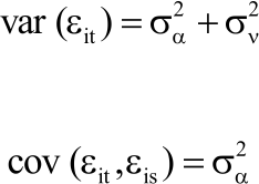 |
Therefore:
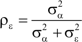 |
Rho is the interclass correlation of the error or the fraction of the variance in the error term due to individual-specific effects. These variables approach 1 if individual effects dominate the idiosyncratic error9,10.
Hausman test: The null hypothesis of the Hausman test is that the preferred model includes random effects and not fixed effects. This test determines whether the unique error (αi) is correlated with the regressor and the null hypothesis is that they are not correlated. The random-effects estimator is highly efficient, so it should be used if the Hausman test supports it. The Hausman test statistic can be calculated only for time-varying regressors and is given as follows14:
 |
Here, RE and FE are the vector of parameter estimates of random effect and fixed effect, respectively. Under the null hypothesis, this statistic has asymptotically the chi-squared distribution with the number of degrees of freedom equal to the rank of the matrix:
 |
Wald test: The Wald test can determine which model variables make significant contributions. The Wald test (also called the Wald chi-squared test) is a way to determine if explanatory variables in a model are significant, meaning that they add something to the model, variables that add nothing can be deleted without affecting the model in a meaningful way. The test can be used for a multitude of different models, including those with binary variables or continuous variables. The null hypothesis for the test is some parameter = some value.
Breusch-pagan lagrange multiplier test: The Breusch-Pagan-Godfrey test is a Lagrange multiplier test of the null hypothesis of no heteroskedasticity, i.e., constant variance among residuals.
Ho: The null hypothesis of the test states that there is constant variance among residuals.
RESULTS AND DISCUSSION
The results obtained in this paper based on applying different statistical tools related to panel regression models are discussed in subsequent sections. This is the first kind of work based on COVID-19 infected case data sets.
Summary statistics: The results presented in Table 1 revealed that the highest number of COVID-19 infected cases was registered in Kanyakumari (118), followed by Tirunelveli (86), Thoothukudi (77) and Tenkasi (49) districts. The lowest number of COVID-19 cases registered in Tenkasi (3) was followed by Thoothukudi (17), Tirunelveli (15) and Kanyakumari (25) districts. In all four districts, the number of COVID-19-infected cases follows a normal distribution since the Jarque-Bera statistical values are non-significant at the 5% level of significance.
Category wise statistics: The categorical number of COVID-19-infected cases is given at the bottom of Table 1. The results show that the number of infected cases in category (0 50) is 7 days in the Kanyakumari district, 31 days in Tenkasi, 15 days each in Thoothukudi and Tirunelveli districts. In the case of (50 100), category 22 days in Kanyakumari district and 16 days in each of the Thoothukudi and Tirunelveli districts, whereas the number of cases registered in the category of (100 150), is 2 days in Kanyakumari districts only.
Figure 1a depicted the total number of COVID-19 cases in all four districts in October, 2020. The highest number of COVID-19-infected cases (2199) was registered in the Kanyakumari district, followed by Thoothukudi (1583), Tirunelveli (1523) and Tenkasi (484). In the Tenkasi district, it is exceptionally low due to more awareness among the people and the district administration might have taken more precautionary measures to prevent COVID-19 infections.
In Kanyakumari District, Fig. 1b depicts that on the 1st and 4th October, 2020, the highest numbers of COVID-19 infected cases registered were 118 and 117, respectively and then they started to decline to 25 cases on 31st October, 2020. Step declining trends have been noted in this district.
Rajarathinam et al.1 reported that Holt’s linear exponential smoothing with α = 0.1413 and β = 0.1071 exhibited a declining trend in the number of infected cases in the Kanyakumari district during the period from 1st August, to 31st December, 2020. The present result also in agreement with this result.
Yongmei and Gao2 by using data-driven modelling reported that evaluation of COVID-19 in Italy decrease due to stay-at-home orders and tracing quarantine interventions.
Roy and Bhattacharya3, also asserted that the imposition of a countrywide lockdown plays an especially important role in restraining the spread of COVID-19 infections.
In the case of Tenkasi District, Fig. 1c showed that the highest number of COVID-19 infected cases registered on 1st October, 2020 decreased to 4 cases on 30th October and then increased to 10 cases at the end of the month. Additionally, in 14 days, only single-digit numbers of infected cases were registered. Upward and downward trends were noted in this district.
Rajarathinam et al.1 reported that Auto-Regressive Integrated Moving Average Model ARIMA (0,1,1) exhibited upward, downward followed by steep declining trend in the number of infected cases in Tenkasi district and this result aligned with current result.
Figure 1d of Thoothukudi District depicts that the highest number of 77 cases registered on 9th October decreased to 42 cases at the end of the month. Very peculiar upward and downward trends have been observed in this district.
In the case of Tirunelveli District, Fig. 1e depicts a stepwise declining trend, with the highest number of 86 infected cases on 1st October, directly declining to 15 at the end of the month.
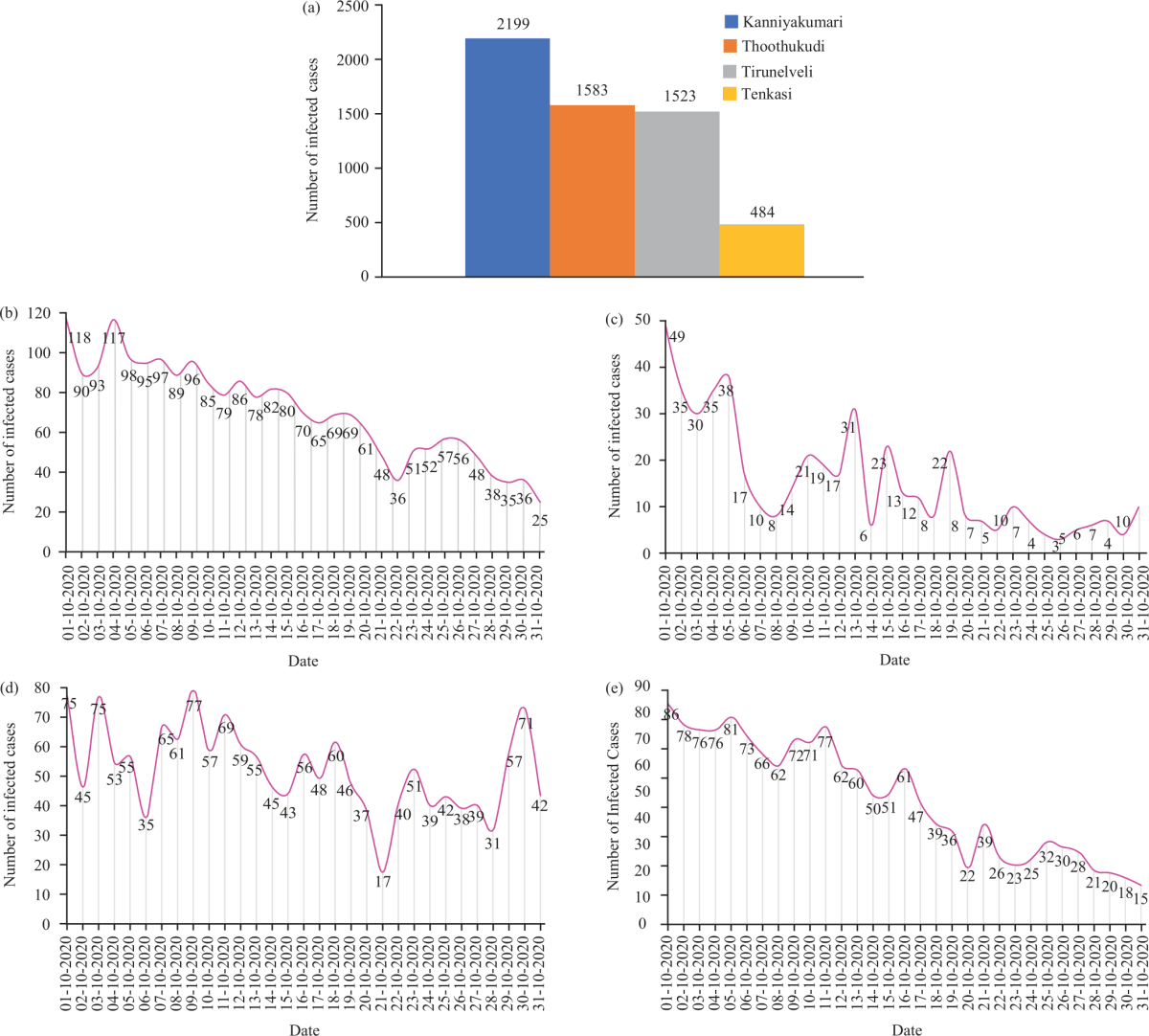 |
| Fig. 1(a-e): | (a) Total number of covid-19 infected cases in all four districts in october 2020, (b) Daily COVID-19 infected cases in Kanyakumari district, (c) Tenkasi district, (d) Thoothukudi district and (e) Tirunelveli district |
| Table 1: Characteristics of summary and category wise statistics | ||||
| Statistics | Kanyakumari | Tenkasi | Thoothukudi | Tirunelveli |
| Mean | 70.93548 | 15.61290 | 51.06452 | 49.12903 |
| Median | 70.00000 | 10.00000 | 51.00000 | 50.00000 |
| Maximum | 118.0000 | 49.00000 | 77.00000 | 86.00000 |
| Minimum | 25.00000 | 3.000000 | 17.00000 | 15.00000 |
| Std. dev. | 24.61156 | 11.97686 | 14.19374 | 22.86007 |
| Skewness | -0.019244 | 1.131092 | -0.001396 | 0.023114 |
| Kurtosis | 2.154139 | 3.372580 | 2.676387 | 1.508788 |
| Jarque-bera | 0.926077 | 6.789374 | 0.135281 | 2.875059 |
| Probability | 0.629368 | 0.033551 | 0.934597 | 0.237514 |
| Sum | 2199.000 | 484.0000 | 1583.000 | 1523.000 |
| Sum sq. dev. | 2199.000 | 4303.355 | 6043.871 | 15677.48 |
| Category | No. of cases | ||||
| (0 50) | 7 | 31 | 15 | 15 | 68 |
| (50 100) | 22 | 0 | 16 | 16 | 58 |
| (100 150) | 2 | 0 | 0 | 0 | 2 |
| Table 2: Analysis of variance test for equality of means for NCASE | |||
| Method | df | Value | Probability |
| ANOVA F-test | (3, 120) | 44.29316 | 0.0000 |
| Welch F-test* | (3, 64.3377) | 64.31809 | 0.0000 |
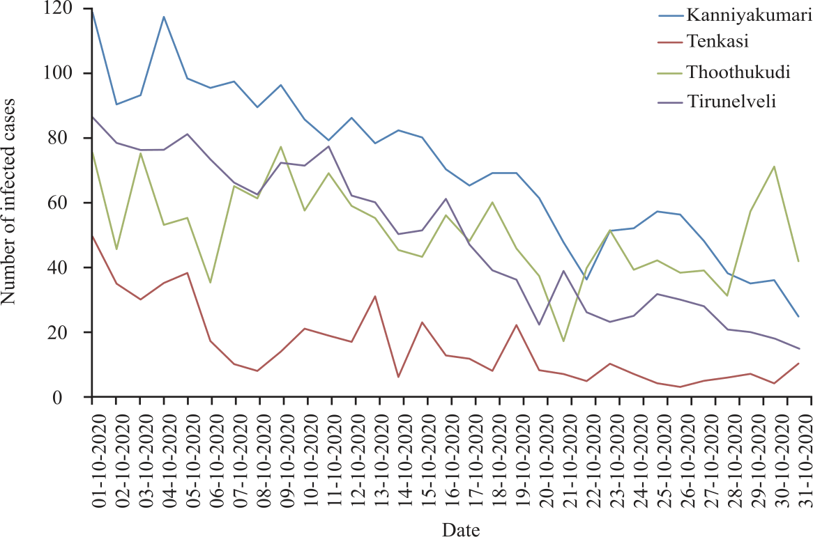 |
| Fig. 2: | Comparisons of COVID-19 infection trends in all four districts |
The pattern of COVID-19-infected cases of Kanyakumari and Tirunelveli followed a similar declining trend, whereas the same upward and downward trend were noted in the cases of Tenkasi and Thoothukudi.
Figure 2 depicts the dates-wise comparison of trends exhibited in the four districts, in which the trend cure of Tenkasi District is at a lower level, followed by those of Thoothukudi, Tirunelveli and Kanyakumari. From this trend pattern, it is noticeably clear that the highest number of infected cases is registered in the Kanyakumari District and the least number of registered cases in the Tenkasi District.
The results presented in Table 2 reveal that the ANOVA F-test value 44, 29316 and Welch F-test value (64.31809) with a p-value = 0.0000 indicate that both tests are highly significant at the 1% level of significance, indicating that the number of COVID-19-infected cases is different from one district to another district (cross-section).
Based on Rajarathinam et al.1 results the above ANOVA test results are ascertained because, Kanyakumari district follow Holt’s linear exponential smoothing trend whereas, in the cases of Tenkasi, Thoothukudi and Tirunelveli exhibited trends are ARIM (0,1,1), ARIMA (2,0,0), ARIMA (2,2,2), respectively. These results reveal that the pattern of COVID-19 infection differs from one district to another.
Takele7 also employed the ARIMA modelling approach for projecting coronavirus (COVID-19) prevalence patterns in East Africa Countries, mainly Ethiopia, Djibouti, Sudan and Somalia.
| Table 3: Characteristics of the unit root test | ||
| Method | Statistic | Prob.** |
| Levin, lin and chu t* | -3.76884 | 0.0001 |
| ** Probabilities are computed assuming asymptotic normality | ||
ARIMA (1,2,1), ARIMA (3,1,1) with drift, ARIMA (0,2,2) and ARIMA (2,2,1) models were chosen as the optimal models for predicting coronavirus cases of Ethiopia, Djibouti, Somalia and Sudan respectively. Utilizing those models, a forecast of four-month a heads future scenario COVID-19 prevalence (July until October 30, 2020) has made. These study results are at par with the results of Rajarathinam et al.1.
Unit root test: Before estimating the panel data regression model, it is necessary to determine the stationary of the variable under study. The unit root test result presented in Table 3 revealed that since the Levin, Lin and Chu t statistics value -3.76884 is significant at the 1% level of significance since the p-value is 0.0001 and hence the study variable, NCASE, is stationary at the level, the variable is I (0).
Takele7 employed Augmented Dickey-Fuller (ADF) test to check the stationary of the daily time series data of Nobel Coronavirus (COVID-19) of Ethiopia, Sudan, Djibouti and Somalia from 13 March-June, 30, 2020. In the current study, the data type is time series of panel type and hence Levin, Lin and Chu t-test is employed.
Constant coefficient model (panel OLS): The CCM method is employed considering the number of new cases (NCASE) as the dependent variable and X, time as the independent variables, the results are presented in Table 4. The result reveals that the intercepts and slopes are highly significant at the 1% level of significance. The slope is negative, which indicates that the number of COVID-19-infected cases decreased by 1.68% in October, 2020. The model is highly significant at the 1% level of significance with an incredibly low R2 value of 29%. Additionally, the estimated Durbin-Watson value of 0.242273 is quite low, which suggests the presence of autocorrelation in the data.
The estimated model assumes that the slope coefficients of time variables X are all identical in all four districts. Therefore, despite its simplicity, the CCM may distort the true relationship between the dependent variable, the number of cases (NCASE) and time, the independent variable X, across the four districts.
Raymundo et al.5 reported that the MGWR model was the most suited in comparison to the OLS (CCM) model in the study of spatial analysis of COVID-19 incidence and the socio-demographic context in Brazil.
| Table 4: Characteristics of the fitted panel least-squares method | ||||
| Variable | Coefficient | Std. error | t-statistic | Prob. |
| C | 73.48710 | 4.257903 | 17.25899 | 0.0000 |
| X | -1.675101 | 0.232288 | -7.211321 | 0.0000 |
| Root MSE | 22.94833 | R-squared | 0.298863 | |
| Mean dependent var. | 46.68548 | Adjusted R-squared | 0.293116 | |
| SD dependent var. | 27.51743 | SE of regression | 23.13566 | |
| Akaike info criterion | 9.136625 | Sum squared residuals | 65301.58 | |
| Schwarz criterion | 9.182114 | Log-likelihood | -564.4708 | |
| Hannan-Quinn criterion | 9.155104 | F-statistic | 52.00315 | |
| Durbin-Watson stat. | 0.242273 | Prob. (F-statistic) | 0.000000 | |
| Table 5: Characteristics of the fixed effects or LSDSV regression model | ||||
Coefficient | Std. error | t-statistic | Prob. | |
| C (1) | 97.7371 | 2.8254 | 34.5913 | 0.0000 |
| C (2) | -1.6751 | 0.1177 | -14.2285 | 0.0000 |
| C (3) | -55.322 | 2.9783 | -18.5751 | 0.0000 |
| C (4) | -19.8709 | 2.9783 | -6.67187 | 0.0000 |
| C (5) | -21.8064 | 2.9783 | -7.32173 | 0.0000 |
| Root MSE | 11.4868 | R-squared | 0.8243 | |
| Mean dependent var. | 46.6854 | Adjusted R-squared | 0.8184 | |
| SD dependent var. | 27.5174 | SE of regression | 11.7256 | |
| Akaike info criterion | 7.80092 | Sum squared residual | 16361.43 | |
| Schwarz criterion | 7.91464 | Log-likelihood | -478.6572 | |
| Hannan-Quinn criterion | 7.84711 | F-statistic | 139.6006 | |
| Durbin-Watson stat. | 0.96695 | Prob (F-statistic) | 0.0000 | |
| Table 6: Cross-section fixed effects values | |
| Crossid | Effect |
| 1 | 24.25000 |
| 2 | -31.07258 |
| 3 | 4.379032 |
| 4 | 2.443548 |
| Table 7: Results of the redundant fixed effects test | |||
| Effects test | Statistic | df | Probability |
| Cross-section F | 118.650551 | (3, 119) | 0.0000 |
| Cross-section chi-square | 171.627101 | 3 | 0.0000 |
| Table 8: Characteristics of the Wald test | |||
| Test statistic | Value | df | Probability |
| F-statistic | 118.6506 | (3, 119) | 0.0000 |
| Chi-square | 355.9517 | 3 | 0.0000 |
Fixed-effect or least-square dummy variable regression model: The results presented in Table 5 reveal that the fixed effect model explains 82% of the variation in the dependent variable. The model is highly significant at the 1% level of significance. The dummy variables were also highly significant at the1% level of significance. The root means square error is 11.4868 with the SE of regression is 11.7256:
NCASE = 97.73701.6751*X-55.3225*(D2)-19.8709*(D3)-21.8064*(D4) |
Based on the statistical significance at the 1% level of significance of the estimated coefficients and the substantial increase in the R2 value to 82% (significant at the 1% level of significance), one can conclude that the fixed effects model or the LSDSV regression model performs better than the panel least-squares regression model (CCM).
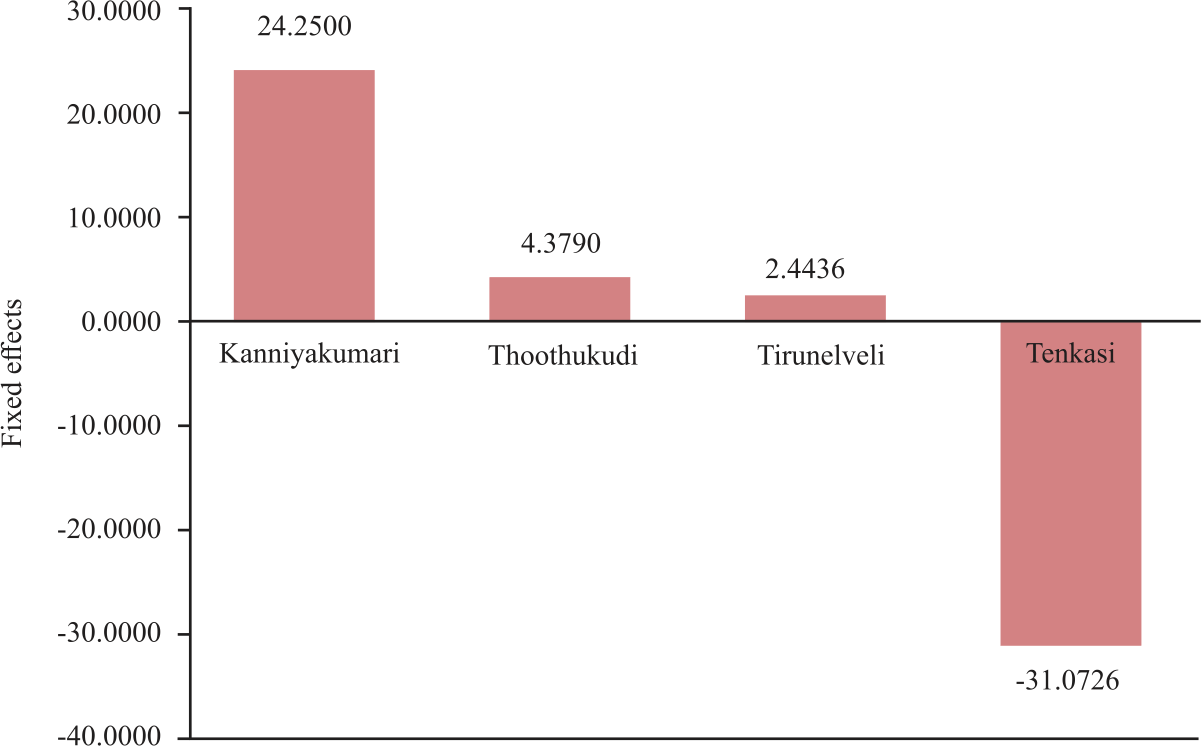
The cross-sectional fixed effects (as deviations from the common intercept) in the context of the fixed effect model are calculated and presented in Table 6. In the Kanyakumari district, 24.2500 is positive and high in comparison to that in the other three districts. This may be due to extremely high infection rates. In the case of Tenkasi District, it is -31.07258, which is extremely exceptionally low. This is because, in this district, an incredibly low rate of infections is noted. In Thoothukudi District, the effect of 4.379032 is exceptionally low in comparison to that of Kanniyakumari District. In the case of Tirunelveli district, it is 2.443548. This fixed effect value is exceptionally low in comparison to that of the Kanyakumari and Thoothukudi districts.
The diagrammatic representation of fixed effects in four different districts is depicted in Fig. 3. Based on this result, it is concluded that the fixed effect model is better than CCM.
To confirm the presence of the fixed effect, the redundant fixed effect test was carried out and the results are presented in Table 7. The test results reveal that the Cross-section F and Chi-square statistics values are significant at the 1% level of significance, indicating that the presence of fixed effects is different from one district to another.
Wald test: To compare the fixed effect model with CCM, the Wald test was carried out. The null hypothesis of the Wald test is H0 = C (3) = C (4) = C (5) = 0, i.e., all three dummy variable values are zero (there is no fixed effect). The result presented in Table 8 reveals that since the F and Chi-square statistics values are significant at the 1% level of significance, the null hypothesis H0 = C (3) = C (4) = C (5) = 0 is rejected, which indicates that the values of the dummy variables are not equal to zero, which confirms fixed effects or the LSDV regression model is an appropriate model in comparison to CCM.
 |
| Fig. 3: | Fixed effect in different districts |
 |
| Fig. 4: | Random effect in different districts |
Oehmke et al.8 also used the Wald test in dynamic panel data modelling to study the surveillance of COVID-19 in the different metropolitan areas in the United States. The test result reveal that the lack of persistence effect is most likely to occur when the number of new cases per day is at a constant speed.
Random-effect model: Finally, the random-effect model is estimated and the results are presented in Table 9. The results reveal that the model is highly significant at the 1% level of significance with an extremely high R2 value of 62% with an SE of regression 1.7257, Root MSE, 11.6307. As in the case of the fixed-effect model, the random-effect model coefficients, intercept and slope are highly significant at the 1% level of significance.
The value of the slope is -1.675101, which is highly significant, indicating that the COVID-19 infection new cases are decreasing at the rate of 1.68%.
Baskar et al.4 reported that the progression of the COVID-19 infection in Tamil Nadu, India is showing decay in the number of infections of the disease which highlights the effectiveness of controlling measures.
The rho value is 0.7915, which indicates that the individual effects of cross-sections are 0.8%.
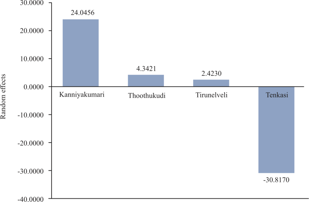
The cross-sectional random effects in the context of the random effect model are calculated and presented in Table 10. The results reveal that in the Kanyakumari district, 24.04562 is positive and high in comparison to that in the other three districts. This may be due to extremely high infection rates. In the case of Tenkasi District, it is -30.81070, which is extremely exceptionally low. This is because of the incredibly low rate of infections in this district. In Thoothukudi District, the effect is 4.342125, which is exceptionally low in comparison to that of Kanniyakumar1 District. In the case of Tirunelveli district, it is 2.422954. This random effect value is exceptionally low in comparison to that of the Kanyakumari and Thoothukudi districts.
The diagrammatic representation of random effects in four different districts is depicted in Fig. 4. Based on this result, the presence of random effects in all four different districts is confirmed.
Breusch-pagan lagrange-multiplier test (heteroskedasticity test): The result presented in Table 11 indicates that the Breusch-Pagan LM test statistic value of 30.35083 and Pesaran scaled LM test statistic value of 7.029479 are highly significant at the 1% level of significance since both statistical p-values are equal to 0.0000, indicating that the null hypothesis of the test, “H0: There is constant variance among residuals”, is rejected. Hence, the above random effect model has the problem of heteroskedasticity.
Hausman test: The Hausman test result presented in Table 12 reveals that the Chi-square statistical value of 0.0000 with 1 degree of freedom is non-significant at a 5% significance level and the null hypothesis “H0: Random Effect Model” is accepted. So, among the three models the random effect model is emerged as the appropriate statistical model to study the trends on COVID-19 daily infected cases.
 |
| Fig. 5: | Confidence interval |
 |
| Fig. 6: | Characteristics of residuals based on the random-effects model Y-axis: Residual values and X-axis: Observed values |
| Table 9: Characteristics of the fitted random effects model | ||||
| Variable | Coefficient | Std. error | t-Statistic | Prob. |
| C | 73.48710 | 11.62358 | 6.322241 | 0.0000 |
| X | -1.675101 | 0.117728 | 14.22852 | 0.0000 |
| Effect specification | SD | Rho |
| Cross-section random | 22.84301 | 0.7915 |
| Idiosyncratic random | 11.72566 | 0.2085 |
| Weighted statistics | |||
| Root MSE | 11.63071 | R-squared | 0.623980 |
| Mean dependent var. | 4.285949 | Adjusted R-squared | 0.620898 |
| SD dependent var. | 19.04403 | SE of regression | 11.72566 |
| Sum squared residual | 16773.90 | F-statistic | 202.4507 |
| Durbin-Watson stat. | 0.943181 | Prob (f-statistic) | 0.000000 |
| Table 10: Cross-section random effects values | |
| Crossid | Effect |
| 1 | 24.04562 |
| 2 | -30.81070 |
| 3 | 4.342125 |
| 4 | 2.422954 |
| Table 11: Characteristics of the residual cross-section dependence test | |||
| Test | Statistic | df | Probability |
| Breusch-pagan LM | 30.35083 | 6 | 0.0000 |
| Pesaran scaled LM | 7.029479 | 0.0000 | |
| Table 12: Characteristics of the hausman test | |||
| Test summary | Chi-sq. statistic | Chi-sq. df | Probability |
| Cross-section random | 0.0000 | 1 | 0.9568 |
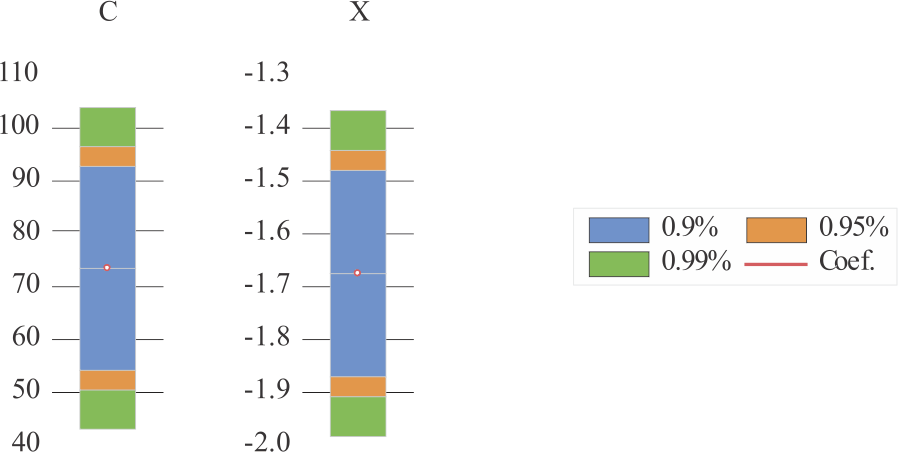
Figure 5 depicts and confirms that the coefficients of intercept and slope lies in the 99% Confidence Interval (CI).
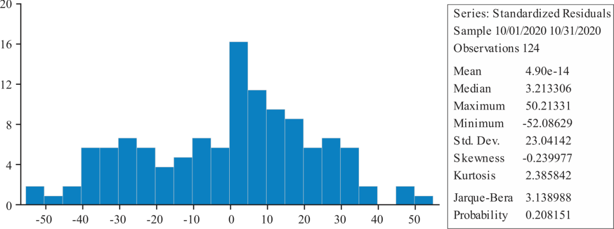
Additionally, Fig. 6 depicted that the residuals are normally distributed because the Jarque-Bera test value is 3.1389, which is found to be non-significant at the 5% level of significance.
This model in future can be extended by taking several other parameters related to age and inclusion of population with the case of respiratory ailments, etc.
CONCLUSION
In this study, the panel data regression model was found to be suitable for assessing the trends in COVID-19-infected cases. The random-effects model was found to be suitable to study the trend. The study results reveal that the highest number of new cases was registered in Kanyakumari, followed by Thoothukudi and Tirunelveli and Tenkasi districts. The lowest number of cases was observed in Tenkasi District. This difference may be due to the precautionary measures taken by the district administration. In general, the trends in the number of COVID-19 infected cases were found to decrease in all four districts by 1.68% in October, 2020.
SIGNIFICANCE STATEMENT
This study revealed that COVID-19-infected cases showed a decreasing trend. The study would be incredibly useful to administrators and decision-makers to take precautionary measures to stop COVID-19 infections. By knowing the COVID-19 infection trends, the academic personal could take appropriate decisions.
REFERENCES
- Rajarathinam, A., P. Tamilselvan and M. Ramji, 2021. Estimating hidden models and trends in COVID-19 infected cases. Strad Res., 8: 128-133.
CrossRefDirect Link - Ding, Y. and L. Gao, 2020. An evaluation of COVID-19 in Italy: A data-driven modeling analysis. Infect. Dis. Modell., 5: 495-501.
CrossRefDirect Link - Roy, S. and K.R. Bhattacharya, 2020. Spread of COVID-19 in India: A mathematical model. J. Sci. Technol., 5: 41-47.
CrossRefDirect Link - Bhaskar, A., C. Ponnuraja, R. Srinivasan and S. Padmanaban, 2020. Distribution and growth rate of COVID-19 outbreak in Tamil nadu: A log-linear regression approach. Indian J. Public Health, 64: 188-191.
CrossRefDirect Link - Raymundo, C.E., M.C. Oliveira, T. de Araujo Eleuterio, S.R. André, M.G. da Silva, E.R. da Silva Queiroz and R. de Andrade Medronho, 2021. Spatial analysis of COVID-19 incidence and the sociodemographic context in Brazil. PLoS ONE, Vol. 16.
CrossRefDirect Link - Bandekar, S.R. and M. Ghosh, 2021. Mathematical modeling of COVID-19 in India and its states with optimal control. Model. Earth Syst. Environ., Vol. 2021.
CrossRefDirect Link - Takele, R., 2020. Stochastic modelling for predicting COVID-19 prevalence in East Africa countries. Infect. Dis. Modell., 5: 598-607.
CrossRefDirect Link - Oehmke, T.B., L.A. Post, C.B. Moss, T.Z. Issa, M.J. Boctor, S.B. Welch and J.F. Oehmke, 2021. Dynamic panel data modeling and surveillance of COVID-19 in metropolitan areas in the united states:Longitudinal trend analysis. J. Med. Internet Res., Vol. 23.
CrossRefDirect Link - Baltagi, B.H., 2021. Econometric Analysis of Panel Data. 6th Edn., Wiley and Sons Ltd., New York, ISBN-13: 978-3-030-53953-5, Pages: 424.
CrossRefDirect Link - Gujarati, D.N., D.C. Porter and G. Sangeetha, 2017. Basic Econometrics. 5th Edn., McGraw-Hill Professional, New York, ISBN-13: 978-0073375779, Pages: 944.
Direct Link - Hsiao, C., 2010. Analysis of Panel Data. 2nd Edn., Cambridge University Press, Cambridge, ISBN-13: 9780511754203, Pages: 366.
Direct Link - Levin, A., C.F. Lin and C.S.J. Chu, 2002. Unit root tests in panel data: Asymptotic and finite-sample properties. J. Econ., 108: 1-24.
CrossRefDirect Link - Hadri, K., 2000. Testing for stationarity in heterogeneous panel data. Econ. J., 3: 148-161.
CrossRefDirect Link - Patrick, R.H., 2020. Durbin–Wu–Hausman specification tests. In: Handbook of Financial Econometrics, Mathematics, Statistics, and Machine Learning. Lee, C.F. and J.C. Lee, World Scientific Publishing Co. Pte. Ltd., Singapore, ISBN-13: 978-981-120-240-7, pp: 1075-1108.
CrossRefDirect Link