
Bruno Montella
Department of Civil, Architectural and Environmental Engineering, Federico II University, Naples, Italy
Luca D`Acierno
Department of Civil, Architectural and Environmental Engineering, Federico II University, Naples, Italy
Mariano Gallo
Department of Engineering, University of Sannio, Italy
Journal of Applied Sciences
Year: 2014 | Volume: 14 | Issue: 21 | Page No.: 2767-2781


ABSTRACT
In this study a model for the optimisation of mass-transit fares is proposed and tested both on a trial and a real-scale network. Formulated as a multidimensional constrained minimisation model, the problem considers a multimodal transportation system under the assumption of elastic demand for simulating the impacts of fare policies on modal split and network performance. It was suggested that the proposed model is applied with the adoption of two objective functions in order to take into account all system and social costs: Firm costs and external costs. Numerical tests show that the main constraints in fare definition are related to the size of public transport subsidies provided by public administration.
PDF Abstract XML References Citation
Received: February 24, 2014;
Accepted: July 15, 2014;
Published: August 16, 2014
How to cite this article
Bruno Montella, Luca D`Acierno and Mariano Gallo, 2014. A Multimodal Approach for Determining Optimal Public Transport Fares. Journal of Applied Sciences, 14: 2767-2781.
DOI: 10.3923/jas.2014.2767.2781
URL: https://scialert.net/abstract/?doi=jas.2014.2767.2781
DOI: 10.3923/jas.2014.2767.2781
URL: https://scialert.net/abstract/?doi=jas.2014.2767.2781
INTRODUCTION
Fares for mass-transit services are generally set below the profitability threshold: Ticket revenues cover only a (minor) part of operational costs while the other part is subsidised by public funds (details on methodologies for calculating public transport subsidies can be found, for instance, in the study of Hao et al. (2009), Yang et al. (2010) and Tscharaktschiew and Hirte (2012). Such fare policies are adopted for social and environmental reasons. Social aspects of the problem have been explored by Chapleau (1995), Hodge (1998), Obeng (2000), Parry and Bento (2002), Paulley et al. (2006), Abrate et al. (2009), Nuworsoo et al. (2009), Attard (2012) and Kallbekken et al. (2013). More generally, the effects of mass-transit pricing policies have been studied by Ballou and Mohan (1981), Ferrari (1999), Karlaftis and McCarthy (2002), Zhang et al. (2006), Jansson (2008), Proost and van Dender (2008) and Basso and Jara-Diaz (2012).
In this study, an optimisation model for establishing mass-transit fares is proposed. In accordance with the problem characteristics, the model satisfies the following requirements:
| • | It assumes transportation demand as elastic, for simulating changes in modal split |
| • | It simulates road and mass-transit transportation systems jointly, to take into account effects of modal split changes on congestion |
| • | It considers different user classes with different socio-economic attributes |
| • | It assumes an objective function that considers all costs: Operational costs, user costs of both road and mass-transit systems and external costs |
Therefore, this problem can be seen as a multimodal network design problem (Montella et al., 2000; D’Acierno et al., 2011a; Cipriani et al., 2012) in which mass-transit fares assume the role of decision variables. A general formulation of the pricing problem was provided by Cascetta (2009) and the multimodal nature of the analysed problem was highlighted by Huang (2000), Casello (2006), Chien and Tsai (2007), Gallo et al. (2011a, b), Gkritza et al. (2011) and Basso and Jara-Diaz (2012). Finally, Osula (1998) showed how changes in mass-transit fares can also modify trip generation.
GENERAL SOLUTION APPROACH
Generally, establishing public transport fares may requires five phases (Fig. 1) that can differ according to the concerned study area. In the area identification phase the area covered by the mass-transit services under study is identified; it can be a city, or part of it, a province or a region. The fare zone definition phase consists of subdividing the territorial area into zones if it is so large that fares have to be differentiated by trip length. The zones should take account of administrative divisions, land uses, pre-existing fare regulations and user perception of fared zones. The mass-transit fare optimisation phase searches for the optimal configuration of mass-transit fares and is the focus of this study. Evaluation of results can suggest modifications to area zoning, by comparing different results the best zoning-fare combination can be identified.
FARE ZONE DEFINITION
If the area is so large that it is not fair to fix the same fare for all trips, the area has to be subdivided into fare zones. This is common practice in metropolitan areas, provinces and regions.
 | |
| Fig. 1: | General approach to mass-transit fare optimisation |
Several methods have been proposed in this respect, based on distances (Cervero, 1982; Daskin et al., 1988; Clark et al., 2011; Borndorfer et al., 2012), time intervals (Cervero, 1981), average travel times (Phillips and Sanders, 1999) or number of zones crossed (Schobel, 2006; Sharaby and Shiftan, 2012). However, three main methods of fare zoning can be identified (Fig. 2): Concentric zones, circular rings and sector zones and alveolar zones.
Concentric zones are mainly adopted where there is a major centre that attracts and/or generates most trips (e.g., a capital city). In this case, also fares for tangential trips are provided. If such trips are considerable, circular rings and sector zones are more commonly used. In this case fares depend on the number of zones crossed. Finally, when there is no major centre, the area can be subdivided into alveolar zones: Fares depend on the number of crossed zones as well.
Although, theoretically speaking, each fare can be independent of the others, in general each fare can be defined according to the minimum fare, that is the fare of a trip within a single zone and the number of crossed zones. This relation can be expressed as:
| (1) |
where, Tb is the mass-transit fare matrix of dimensions (nTicketsxnMaxCrossedZones), whose generic element tin is the fare of the i-th ticket type that allows up to n zones to be crossed; tb0 is the vector of basic mass-transit fare of dimensions (nTicketsx1), whose elements ti0 are the first row elements of matrix Tb and represent fares that allow travel only within the same zone (intra-zonal trips); 1 is a vector of dimensions (nTicketsx1), whose elements are all equal to 1; tb* is the vector of basic variation in fares of dimensions (nTicketsx1), whose elements represent the unit variation in fares without considering any corrective coefficient; A is the corrective coefficient matrix of dimensions (nTicketsxnMaxCrossedZones), whose generic element ain is a corrective coefficient related to the i-th ticket type that allows up to n zones to be crossed; N is a vector of dimensions (nMaxCrossedZonesx1), whose generic element nj is equal to (j-1).
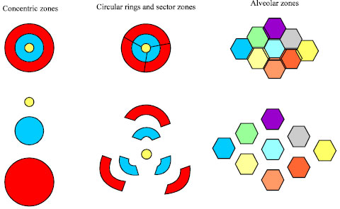 | |
| Fig. 2: | Types of fare zone |
Equation 1 is equivalent to the following:
| (2) |
where, Γ is a matrix of dimensions (nTicketsxnMaxCrossedZones), whose generic element γin is a coefficient related to the i-th ticket type that allows up to n zones to be crossed.
Indeed, since both previous equations are linear, assuming:
where, A* is a vector whose generic element ai* is equal to the ratio between ti* and ti0, Eq. 1 may be transformed into Eq. 2 via the following relation:
| (3) |
where,![]() is a matrix of dimensions (nTicketsxnMaxCrossedZones), whose elements are all equal to 1.
is a matrix of dimensions (nTicketsxnMaxCrossedZones), whose elements are all equal to 1.
Thus, we proposed to adopt Eq. 2 for defining fare zone criteria using the matrix Γ as the only parameter.
MASS-TRANSIT FARE OPTIMISATION MODEL
The proposed mass-transit fare optimisation model can be formulated as follows:
| (4) |
Subject to:
| (5) |
| (6) |
| (7) |
where, ![]() is the optimal value for Tb,
is the optimal value for Tb, ![]() is the feasibility set of matrices Tb, Z(·) is the objective function to be minimised, fc* is the equilibrium link flow matrix for the road system of dimensions (nRoadLinksxnUserCategories), fb* is the equilibrium link flow matrix for the mass-transit system of dimensions (nTransitLinksxnUserCategories), Λ(·) is the multimode assignment function which provides equilibrium flows as a solution of a fixed-point problem, TR is the monetary value obtained by selling public transport tickets, generally indicated as mass-transit revenues which obviously depends on fare values (Tb) and number of mass-transit system users (fb*), α is a term which expresses the part of operational costs not covered by subsidies, B is the budget used for implementing the mass-transit system, generally equal to the total operational cost,
is the feasibility set of matrices Tb, Z(·) is the objective function to be minimised, fc* is the equilibrium link flow matrix for the road system of dimensions (nRoadLinksxnUserCategories), fb* is the equilibrium link flow matrix for the mass-transit system of dimensions (nTransitLinksxnUserCategories), Λ(·) is the multimode assignment function which provides equilibrium flows as a solution of a fixed-point problem, TR is the monetary value obtained by selling public transport tickets, generally indicated as mass-transit revenues which obviously depends on fare values (Tb) and number of mass-transit system users (fb*), α is a term which expresses the part of operational costs not covered by subsidies, B is the budget used for implementing the mass-transit system, generally equal to the total operational cost, ![]() is the feasibility set for fc* and
is the feasibility set for fc* and ![]() is the feasibility set for fb*.
is the feasibility set for fb*.
Constraint (Eq. 5) represents the multimodal equilibrium assignment; it constrains road and mass-transit flows to be in multimodal equilibrium for each configuration of mass-transit fares, Tb. Equilibrium flows can be calculated by means of three kinds of models: Supply, demand and flow propagation models.
Supply models describe the performance of transportation systems in relation to user flows (e.g., an increase in vehicles on a road generally produces an increase in travel times). Such models (Cascetta, 2009) can be formulated by means of the following equation:
| (8) |
where, Cim is the vector of generalised path costs associated to mode m (where m = c in the case of road systems and m = b in the case of mass-transit systems) for user category i, of dimensions (nRoadPathsx1) in the case of road systems and (nTransitHyperpathsx1) in the case of mass-transit systems. Indeed, in the case of mass-transit systems, we adopt the hyperpath approach proposed by Nguyen et al. (1998) in order to simulate preventive-adaptive choice behaviours since users are unable to set their itineraries preventively. Indeed, since the physical path depends on the arrival of vehicles at boarding stops, users choose the set of attractive lines beforehand (preventive stage) and the line used according to arrival events (adaptive stage), Δm,i is the link-path (or link-hyperpath) incidence matrix associated to mode m for user category i, whose generic element ![]() is equal to 1 if link l belongs to path (or hyperpath) k, 0 otherwise, of dimensions (nRoadLinksxnRoadPaths) in the case of the road system and (nTransitLinksxnTransitHyperaths) in the case of the mass-transit system; cim is the vector of generalised link costs associated to mode m for user category i, of dimensions (nRoadLinksx1) in the case of the road system and (nTransitLinksx1) for the mass-transit system, fc is the vector of generic link flow associated to the road system, of dimensions (nRoadLinksx1), fb is the vector of generic link flow associated to the mass-transit system, of dimensions (nTransitLinksx1),
is equal to 1 if link l belongs to path (or hyperpath) k, 0 otherwise, of dimensions (nRoadLinksxnRoadPaths) in the case of the road system and (nTransitLinksxnTransitHyperaths) in the case of the mass-transit system; cim is the vector of generalised link costs associated to mode m for user category i, of dimensions (nRoadLinksx1) in the case of the road system and (nTransitLinksx1) for the mass-transit system, fc is the vector of generic link flow associated to the road system, of dimensions (nRoadLinksx1), fb is the vector of generic link flow associated to the mass-transit system, of dimensions (nTransitLinksx1), ![]() is the vector of non-additive path costs associated to mode m for user category i, whose generic element
is the vector of non-additive path costs associated to mode m for user category i, whose generic element ![]() expresses costs that depend only on path k (such as road tolls at motorway entrance/exit points in the case of the road system and waiting time at bus stops/train stations or fares for the mass-transit system), of dimension (nRoadPathsx1) for the road system and (nTransitHyperpathsx1) for the mass-transit system. Therefore, path cost vectors for the road system can be assumed as constants while in the case of the mass-transit system they have to be assumed at least as a function of vector Tb, that is:
expresses costs that depend only on path k (such as road tolls at motorway entrance/exit points in the case of the road system and waiting time at bus stops/train stations or fares for the mass-transit system), of dimension (nRoadPathsx1) for the road system and (nTransitHyperpathsx1) for the mass-transit system. Therefore, path cost vectors for the road system can be assumed as constants while in the case of the mass-transit system they have to be assumed at least as a function of vector Tb, that is:
Likewise, demand models imitate user choices influenced by transportation system performance. In particular, these models are based on the assumption that users are rational decision makers maximising utility (or equivalently, minimising generalized costs) through their choices. These models can be formulated by means of the following equation:
| (9) |
where, ![]() is the vector of path (or hyperpath) flows associated to mode m for user category i, of dimensions (nRoadPathsx1) for the road system and (nTransitHyperpathsx1) for mass-transit; Pim is the matrix of path (or hyperpath) choice probabilities associated to mode m for user category i, whose generic element
is the vector of path (or hyperpath) flows associated to mode m for user category i, of dimensions (nRoadPathsx1) for the road system and (nTransitHyperpathsx1) for mass-transit; Pim is the matrix of path (or hyperpath) choice probabilities associated to mode m for user category i, whose generic element ![]() expresses the probability of people travelling between origin o and destination d on path (or hyperpath) k, of dimensions (nRoadPathsxnOriginDestinationPairs) for the road system and (nTransitHyperpathsxnOriginDestinationPairs) for mass-transit system; dim is the vector of travel demand associated to mode m for user category i, whose generic element
expresses the probability of people travelling between origin o and destination d on path (or hyperpath) k, of dimensions (nRoadPathsxnOriginDestinationPairs) for the road system and (nTransitHyperpathsxnOriginDestinationPairs) for mass-transit system; dim is the vector of travel demand associated to mode m for user category i, whose generic element ![]() expresses the average number of users travelling between origin o and destination d in a time unit, of dimensions (nOriginDestinationPairsx1).
expresses the average number of users travelling between origin o and destination d in a time unit, of dimensions (nOriginDestinationPairsx1).
It is worth noting that matrix Pim depends only on path costs of the same transportation system while vector dim depends on path costs of all transportation systems.
Flow propagation models describe the relation between path costs and link flows. In particular, with the assumption of intra-period stationarity, such models can be expressed as:
| (10) |
Since the flow on a link can be expressed as the sum of all flows on the same link belonging to different user categories, that is:
| (11) |
The interaction between supply, demand and flow propagation models, in order to obtain equilibrium flows, provides the following equation:
| (12) |
By splitting Eq. 12 for each transportation system and explicitly expressing the dependence of mass-transit non-additive hyperpath costs on mass-transit fares, we obtain the following fixed-point formulation (Cantarella, 1997; D'Acierno et al., 2011b):
 | (13) |
which can be reduced to:
that is constraint (Eq. 5). The solution of the fixed-point problem (Eq. 13) or equivalently (Eq. 5), consists in obtaining road and mass-transit flows which generate road and mass-transit generalised costs that produce a modal split and path choices such that the same flows are reproduced. For solving the multimodal equilibrium assignment problem, in this study we adopt the fixed-point model and the solution algorithms proposed by D’Acierno et al. (2011b).
Under constraint (Eq. 6) ticket revenues have to cover at least the share of operational costs which is not subsidised by public authorities. According to constraint (Eq. 7) flows have to belong to feasibility sets that express consistency of flows (for instance, the sum of all ingoing flows in a node has to be equal to the sum of all outgoing flows if the node is not a centroid).
Since the calculation and check of Eq. 5 requires implementation of suitable algorithms, the proposed model shows a bi-level formulation: The upper level is the optimisation model (Eq. 4) and the lower is the assignment problem (Eq. 5) subject to Eq. 7. Therefore, if matrix Γ is fixed, through Eq. 2, the optimisation model (Eq. 4) can be simplified as:
Upper level:
| (14) |
Subject to:
| (15) |
Lower level:
| (16) |
Subject to:
| (17) |
where, ![]() is the optimal value and
is the optimal value and ![]() the feasibility set of tb0. This second model (Eq. 14-17) has less complexity since vector tb0 has only nTickets elements, while matrix Tb has nTicketsxnMaxCrossedZones elements to be optimised.
the feasibility set of tb0. This second model (Eq. 14-17) has less complexity since vector tb0 has only nTickets elements, while matrix Tb has nTicketsxnMaxCrossedZones elements to be optimised.
In this study, two objective functions are tested; the first is the objective function adopted in several mass-transit network design problems that considers only system costs and user costs, adapted to our multimodal problem:
| (18) |
where, NOTC(·) is the Net Operational Transit Cost and UGC(·) is the User Generalised Cost of all transportation systems.
The NOTC term can be expressed as the difference between the Total Operational Transit Cost (TOTC) and Ticket Revenue (TR), that is:
| (19) |
In particular, we proposed to adopt the following formulations:
| (20) |
| (21) |
where, ![]() is the standard cost per kilometre of line λ, expressed in euro/km; Lλ is the length of line λ, expressed in km; φλ is the service frequency of line λ, expressed in buses/h or trains/h;
is the standard cost per kilometre of line λ, expressed in euro/km; Lλ is the length of line λ, expressed in km; φλ is the service frequency of line λ, expressed in buses/h or trains/h; ![]() is the average number of users of the mass-transit system, belonging to user category i, travelling from origin o to destination d, expressed in users/h;
is the average number of users of the mass-transit system, belonging to user category i, travelling from origin o to destination d, expressed in users/h; ![]() is the value of the ticket for user category i entitling him/her to travel from origin o to destination d, expressed in Euros.
is the value of the ticket for user category i entitling him/her to travel from origin o to destination d, expressed in Euros.
The UGC term can be expressed as the sum of the Road System User Cost (RSUC) and Transit System User Cost (TSUC), that is:
| (22) |
With:
| (23) |
 | (24) |
where, ![]() is the vector of waiting times of mass-transit system users belonging to category i, whose generic element Twib,k expresses the average total waiting time at bus stops/train stations spent by users travelling along hyperpath k, of dimensions (nTransitHyperpathsx1).
is the vector of waiting times of mass-transit system users belonging to category i, whose generic element Twib,k expresses the average total waiting time at bus stops/train stations spent by users travelling along hyperpath k, of dimensions (nTransitHyperpathsx1).
We expressed the non-additive hyperpath cost for the mass-transit system by splitting waiting time and ticket costs in order to show that in the objective function (Eq. 18) the term TR has both a positive (namely mass-transit system revenues) and negative (ticket costs) sign. Hence, it can be omitted. Therefore, mass-transit fares in the proposed optimisation model do not appear explicitly in the cost function formulation but implicitly by means of assignment (Eq. 5) and budget (Eq. 6) constraints.
Moreover, we propose to adopt a second objective function which also considers external costs, EC(·), produced by road traffic, that is:
| (25) |
Also in this second case mass-transit revenues and ticket costs for users are not present since they cancel each other out. Details on external cost formulation adopted in this model can be found in a Gallo et al. (2011a), where the same numerical parameters are applied in a real scale network.
NUMERICAL APPLICATIONS
The proposed model was tested on a trial network and on a real-scale network. The descriptions of networks and results of the tests are reported as follows.
 | |
| Fig. 3: | Simple network framework |
Trial network: The proposed optimisation model was tested on the simple network of Fig. 3, where, neglecting Eq. 6 (or equivalently Eq. 15) the problem may be solved in a closed form; this network has one link, a, shared by road and mass-transit systems and there is a single bus line l. Moreover, it is assumed that there is a single fare zone, a single ticket type, a single user category and hence a single fare, ![]()
The Total Operational Transit Cost (TOTC) is calculated as:
| (26) |
where, cloc is the unit operational cost of line l, Ll is the length of line l and φl is the service frequency of line l.
Road System User Cost (RSUC) on the link is equal to the sum of user travel times, indicated as UTCc,a and expressed by means of cost function ca (fc,a) and the Road Monetary Costs (road/parking pricing), RMCa, applied on the link.
Likewise the User Transit System User Cost is equal to the sum of user travel times, indicated as UTCb,a and the mass-transit ticket cost tb0. In particular, UTCb,a is equal to the sum of the on-board time, assumed equal to the road travel time, ca(fc, a), the waiting time, equal to the ratio between a regularity term ηl and the frequency φl of the line and the access-egress time, cp, that is:
| (27) |
The mode choice model is expressed by means of a Multinomial Logit model, where the systematic utility of road and mass-transit users, indicated as Vc and Vb, are as follows:
| (28) |
| (29) |
where, MSEc and MSEb are the socio-economic variables of modal choice model, respectively for the road and mass-transit system. Moreover, the β terms are the parameters of the model. Therefore the road travel demand can be estimated as:
 | (30) |
and the mass-transit travel demand is:
| (31) |
Assuming that capacity constraints are not present on the mass-transit system, the mass-transit (user) flow, fb,a, is equal to the mass-transit demand, db; moreover, the road (vehicle) flow, fc,a, is equal to the ratio between the road demand, dc and the occupancy index, δc, assumed constant. Therefore, objective function (Eq. 18) can be written as:
 | (32) |
Since objective function (Eq. 32) is continuous with continuous first and second partial derivatives, the road travel time function is continuous with continuous first and second partial derivatives and the feasibility set of mass-transit fares is a closed interval [0, tb0,max], solution ![]() of Eq. 14 is one of the points among endpoints of feasibility interval (i.e., 0 and tb0,max) and values
of Eq. 14 is one of the points among endpoints of feasibility interval (i.e., 0 and tb0,max) and values ![]() (of the above feasibility set) that satisfy conditions:
(of the above feasibility set) that satisfy conditions:
 | (33) |
If road travel time is estimated by means of a BPR function, that is:
| (34) |
Equation 33 may be stated to be satisfied with:
 | (35) |
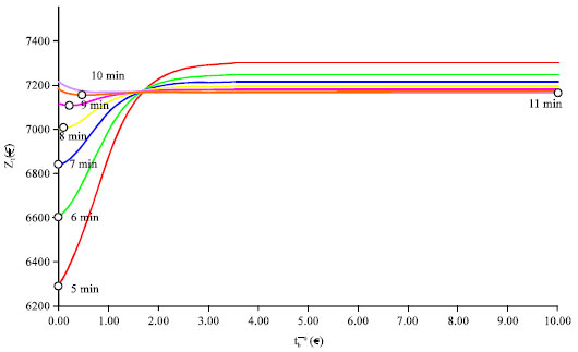 | |
| Fig. 4: | Objective function chart by TWT value |
Only if:
 | (36) |
where, ca0 is the free-flow road travel time on link a, that is equal to the ratio between the length of link a and the free-flow average speed on the same link; αaBPR and βaBPR are parameters of the BPR function; Capa is the capacity of link a. Therefore, if condition of Eq. 36 is not satisfied, the solution of Eq. 14 is one of the endpoints of interval [0, tb0,max].
Adopting the parameters in Table 1, the solution of Eq. 4 may be analysed. In particular, Fig. 4 shows objective function (Eq. 32) by different TWT values, with:
| (37) |
where, the TWT variation is obtained by φl variation.
| Table 1: | Parameter values |
 | |
A major result is that with TWT values lower than 8 min and higher than 10 min the solution is an endpoint of feasibility interval (in this case tb0,max is equal to _10.00). Besides when the solution is a value that puts the first derivative equal to zero, the mass-transit fare increases when the TWT value increases. This means that, when the mass-transit travel time increases with respect to the road travel time, the system optimum (hence the minimum value of the objective function) can be obtained by increasing mass-transit fares and hence moving users from the mass-transit system to the road system. Indeed, although the increase in the number of road users increases both road and mass-transit travel times and hence the objective function value, the decrease in the number of mass-transit users reduces the number of users that incur the Transit Waiting Time (TWT) and yields a decrease in the objective function that counterbalances the increase due to travel time increases.
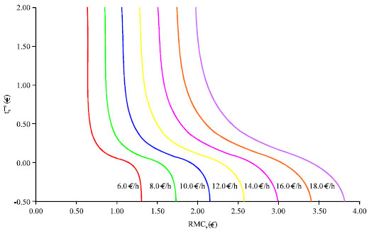
Figure 5 shows that Eq. 35 has an asymptotic trend to endpoints of its feasibility interval (Eq. 36). In this case the TWT variation yields a translation of ![]() and endpoints of Eq. 35, where the difference is equal to the product of the value δc, TWT variation and the ratio between βaTIME and βaCOST.
and endpoints of Eq. 35, where the difference is equal to the product of the value δc, TWT variation and the ratio between βaTIME and βaCOST.
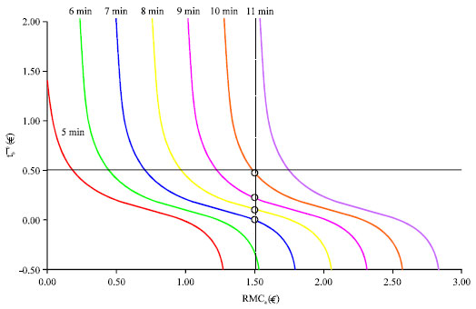 | |
| Fig. 5: | Mass-transit fares by RMCa and TWT values |
 | |
| Fig. 6: | Mass-transit fares by RMCa and values of time |
Another important result is that, in fixing TWT values, an increase in road monetary costs yields a decrease in mass-transit fares. Indeed, an increase in road monetary costs increases the objective function value while a decrease in mass-transit fares yields a decrease in the number of road users that entails a decrease in both road and mass-transit travel times, a reduction in users that have to support road monetary costs and hence a reduction in the objective function value that counterbalances the increase due to the rise in road monetary costs. Finally, the dotted line corresponding to the road monetary cost of _1.50 intercepts curves at solution points in Fig. 4.
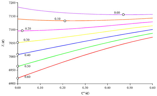
An increase in the ratio between βaTIME and βaCOST (for instance by fixing βaTIME and reducing βaCOST), yields an increase in both the width of the feasibility interval and the mass-transit fare (Fig. 6).
 | |
| Fig. 7: | Objective function chart by βTUV values |
| Table 2: | Real-scale features |
 | |
Introducing the external costs in the objective function, assuming that:
| (38) |
where, βTUV is the Transit User Value that expresses the value that society associates to a user travelling on the mass-transit system, the objective function (Eq. 32) can be written as:
 | (39) |
Also in this case solution ![]() of Eq. 14 is one of the endpoints of the feasibility interval (i.e., 0 and tb0,max) and values
of Eq. 14 is one of the endpoints of the feasibility interval (i.e., 0 and tb0,max) and values ![]() (of the above feasibility set) that satisfy the Eq. 33 for Z2(·).
(of the above feasibility set) that satisfy the Eq. 33 for Z2(·).
Finally, Fig. 7 shows that an increase in term βTUV yields a decrease in mass-transit fares.
Real-scale network: The proposed approach was tested also on a real-scale network (Fig. 8, with features reported in Table 2) in order to ascertain the applicability of the proposed model. In particular, we sought the optimal value of multiplier μ which allows us to:
| • | Modify all existing fares proportionally |
| • | Minimise both the proposed objective functions |
| • | Jointly satisfy assignment and budget constraints |
We developed and implemented a solution algorithm on a PC Intel Core2 Quad Q6600 2.40 Ghz which provided results in 26.3 min (i.e., about 0.8 min per solution examined). Table 3 synthesises cost function terms for each considered multiplier value. Figure 9 shows objective function values depending on the multiplier value, while Figure 10-16 highlight trends in single terms.
Generally, an increase in mass-transit fares will produce a reduction in mass-transit travel demand and an increase in road travel demand. This in turn means an increase in road congestion and related road travel times, fuel consumption and external costs. Mass-transit user costs generally increase with respect to the zero-fare condition because in the case of shared lanes (i.e., buses in a rural context) road congestion will also produce an increase in mass-transit travel times.
Mass-transit user costs could decrease with a reduction in travel demand. However, as regards the average travel cost per user, there could be a decrease since users who chose to modify their mode choice were initially using high cost hyperpaths.
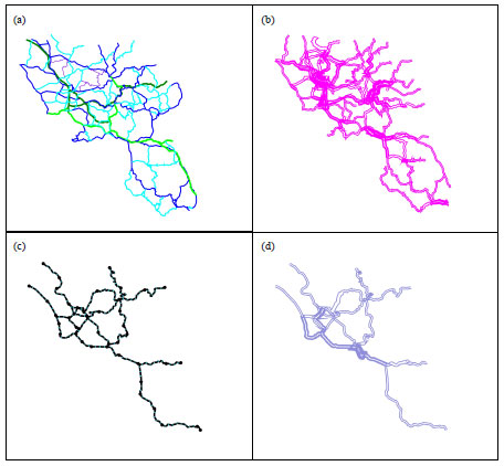 | |
| Fig. 8(a-d): | Real-scale network, (a) Road network, (b) Bus lines, (c) Rail network and (d) Rail lines |
| Table 3: | Real-dimension network application |
 | |
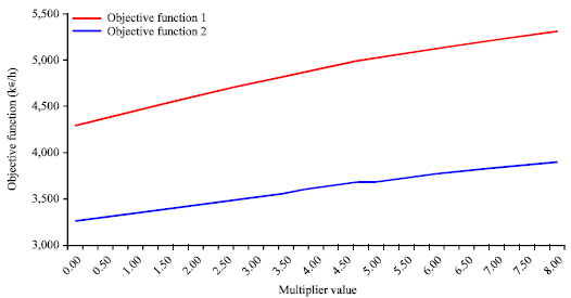 | |
| Fig. 9: | Objective function values |
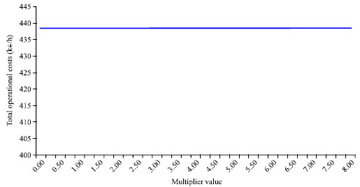 | |
| Fig. 10: | Total operational costs |
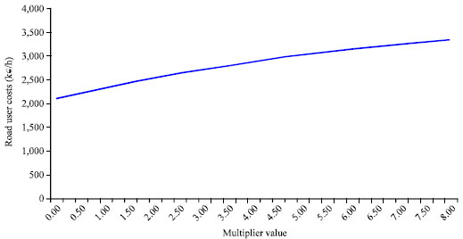 | |
| Fig. 11: | Road user costs |
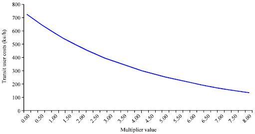 | |
| Fig. 12: | Mass-transit user costs (except ticket costs) |
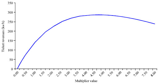 | |
| Fig. 13: | Ticket revenues |
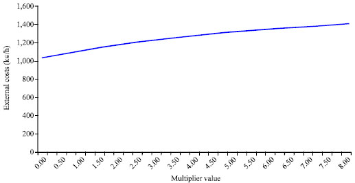 | |
| Fig. 14: | External costs |
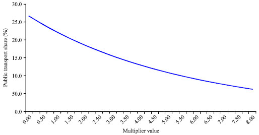 | |
| Fig. 15: | Public transport share |
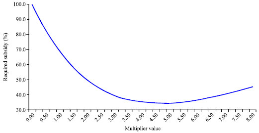 | |
| Fig. 16: | Required subsidy |
Finally, the trend in ticket revenues shows that there is initially an increase in revenues because the reduction in consumers is compensated by the increase in fares. Compensation effects then tend to diminish until a reduction in revenues is produced.
CONCLUSION
In this study we proposed a multimodal and multiuser model for determining optimal mass-transit fares in real contexts. The problem was formulated with a multidimensional constrained minimisation model where constraints are strongly interdependent (e.g., the assignment constraint influences the values of other constraints). The use of a multimodal and multiuser assignment model allows the problem to be broken down into a bi-level problem: The upper level is the optimisation problem with budget constraints and the lower is the assignment problem with consistency constraints.
Application on a trial network highlighted the properties of the problem and testing on a real-scale network showed that the proposed model provides results in reasonable calculation times. However, initial results indicate that the budget constraint greatly affects the optimal solution irrespective of the explicit consideration of external costs. Future research could be directed at testing other real-scale networks in order to ascertain whether budget constraints are, after all, the only parameter to be considered.
ACKNOWLEDGMENT
This study is partially supported under research project PON-DIGITAL PATTERN grant No. PON01_01268.
REFERENCES
- Abrate, G., M. Piacenza and D. Vannoni, 2009. The impact of integrated tariff systems on public transport demand: Evidence from Italy. Reg. Sci. Urban Econ., 39: 120-127.
CrossRefDirect Link - Attard, M., 2012. Reforming the urban public transport bus system in Malta: Approach and acceptance. Trans. Res. Part A: Policy Pract., 46: 981-992.
CrossRefDirect Link - Ballou, D.P. and L. Mohan, 1981. A decision model for evaluating transit pricing policies. Trans. Res. Part A: Gen., 15: 125-138.
CrossRefDirect Link - Basso, L.J. and S.R. Jara-Diaz, 2012. Integrating congestion pricing, transit subsidies and mode choice. Transp. Res. Part A: Policy Pract., 46: 890-900.
CrossRefDirect Link - Borndorfer, R., M. Karbstein and M.E. Pfetsch, 2012. Models for fare planning in public transport. Discrete Applied Math., 160: 2591-2605.
CrossRef - Cantarella, G.E., 1997. A general fixed-point approach to multimode multi-user equilibrium assignment with elastic demand. Trans. Sci., 31: 107-128.
CrossRef - Casello, J.M., 2006. Transit competitiveness in polycentric metropolitan regions. Trans. Res. Part A: Policy Pract., 41: 19-40.
CrossRefDirect Link - Cervero, R., 1981. Flat versus differentiated transit pricing: What's a fair fare. Transportation, 10: 211-232.
CrossRefDirect Link - Cervero, R., 1982. The transit pricing evaluation model: A tool for exploring fare policy options. Trans. Res. Part A: Gen., 16: 313-323.
CrossRefDirect Link - Chien, S.I.J.Y. and C.F.M. Tsai, 2007. Optimization of fare structure and service frequency for maximum profitability of transit systems. Trans. Plann. Technol., 30: 477-500.
CrossRefDirect Link - Cipriani, E., S. Gori and M. Petrelli, 2012. A bus network design procedure with elastic demand for large urban areas. Public Transp., 4: 57-76.
CrossRefDirect Link - Clark, D.J., F. Jorgensen and T.A. Mathisen, 2011. Relationships between fares, trip length and market competition. Trans. Res. Part A: Policy Pract., 5: 611-624.
CrossRefDirect Link - D'Acierno, L., R. Ciccarelli, B. Montella and M. Gallo, 2011. A multimodal multiuser approach for analysing pricing policies in urban contexts. J. Applied Sci., 11: 599-609.
CrossRefDirect Link - D'Acierno, L., M. Gallo and B. Montella, 2011. A fixed-point model and solution algorithms for simulating urban freight distribution in a multimodal context. J. Applied Sci., 11: 647-654.
CrossRefDirect Link - Daskin, M.S., J.L. Schofer and A.E. Haghani, 1988. A quadratic programming model for designing and evaluating distance-based and zone fares for urban transit. Trans. Res. Part B: Methodol., 22: 25-44.
CrossRefDirect Link - Ferrari, P., 1999. A model of urban transport management. Trans. Res. Part B: Methodol., 33: 43-61.
CrossRefDirect Link - Gallo, M., B. Montella and L. D'Acierno, 2011. The transit network design problem with elastic demand and internalisation of external costs: An application to rail frequency optimisation. Transp. Res. Part C: Emerg. Technol., 19: 1276-1305.
CrossRefDirect Link - Gkritza, K., M.G. Karlaftis and F.L. Mannering, 2011. Estimating multimodal transit ridership with a varying fare structure. Trans. Res. Part A: Policy Pract., 5: 148-160.
CrossRefDirect Link - Hao, J., W. Zhou, H. Huang and H. Guan, 2009. Calculating model of urban public transit subsidy. J. Trans. Syst. Eng. Inform. Technol., 9: 11-16.
CrossRef - Hodge, D.C., 1998. Fiscal equity in urban mass transit systems: A geographic analysis. Ann. Assoc. Am. Geographers, 78: 288-306.
CrossRef - Huang, H.J., 2000. Fares and tolls in a competitive system with transit and highway: The case with two groups of commuters. Trans. Res. Part E: Logist. Trans. Rev., 36: 267-284.
CrossRefDirect Link - Jansson, J.O., 2008. Public transport policy for central-city travel in the light of recent experiences of congestion charging. Res. Trans. Econ., 22: 179-187.
CrossRef - Kallbekken, S., J.H. Garcia and K. Korneliussen, 2013. Determinants of public support for transport taxes. Trans. Res. Part A: Policy Pract., 58: 67-78.
CrossRefDirect Link - Karlaftis, M.G. and P. McCarthy, 2002. Cost structures of public transit systems: A panel data analysis. Trans. Res. Part E: Logist. Trans. Rev., 38: 1-18.
CrossRefDirect Link - Nguyen, S., S. Pallottino and M. Gendreau, 1998. Implicit enumeration of hyperpaths in a logit model for transit networks. Transportation Sci., 32: 54-64.
CrossRef - Nuworsoo, C., A. Golub and E. Deakin, 2009. Analyzing equity impacts of transit fare changes: Case study of Alameda-Contra Costa Transit, California. Eval. Program Plann., 32: 360-368.
CrossRefDirect Link - Obeng, K., 2000. Expense preference behavior in public transit systems. Trans. Res. Part E: Logist. Trans. Rev., 36: 249-265.
CrossRefDirect Link - Osula, D.O.A., 1998. A procedure for estimating transit subsidization requirements for developing countries. Trans. Res. Part A: Policy Pract., 32: 599-606.
CrossRefDirect Link - Parry, I.W.H. and A. Bento, 2002. Estimating the welfare effect of congestion taxes: The critical importance of other distortions within the transport system. J. Urban Econ., 51: 339-365.
CrossRefDirect Link - Paulley, N., R. Balcombe, R. Mackett, H. Titheridge and J. Preston et al., 2006. The demand for public transport: The effects of fares, quality of service, income and car ownership. Trans. Policy, 13: 295-306.
CrossRefDirect Link - Phillips, B. and P. Sanders, 1999. Time-based zones: An alternate pricing strategy. J. Prod. Brand Manage., 8: 73-82.
CrossRef - Proost, S. and K. van Dender, 2008. Optimal urban transport pricing in the presence of congestion, economies of density and costly public funds. Trans. Res. Part A: Policy Pract., 42: 1220-1230.
CrossRefDirect Link - Sharaby, N. and Y. Shiftan, 2012. The impact of fare integration on travel behavior and transit ridership. Trans. Policy, 21: 63-70.
CrossRefDirect Link - Tscharaktschiew, S. and G. Hirte, 2012. Should subsidies to urban passenger transport be increased? A spatial CGE analysis for a German metropolitan area. Trans. Res. Part A: Policy Pract., 46: 285-309.
CrossRefDirect Link - Yang, Y., K. Qi, K. Qian, Q. Xu and L. Yang, 2010. Public transport subsidies based on passenger volume. J. Trans. Syst. Eng. Inform. Technol., 10: 69-74.
CrossRefDirect Link - Zhang, X., N. Paulley, M. Hudson and G. Rhys-Tyler, 2006. A method for the design of optimal transport strategies. Trans. Policy, 13: 329-338.
CrossRefDirect Link