
Lei Zhang
Chongqing Special Equipment Inspection and Research Institute, 401121, Chongqing, China
Xiao Lv
Chongqing Special Equipment Inspection and Research Institute, 401121, Chongqing, China
Li Zhang
Chongqing Special Equipment Inspection and Research Institute, 401121, Chongqing, China
Journal of Applied Sciences
Year: 2014 | Volume: 14 | Issue: 19 | Page No.: 2367-2373


ABSTRACT
This study presents a characteristic analysis based on stroboscopic mapping modeling method and fixed points theory in current-fed Contactless Power Transfer (CPT) system. Circulation influence of resonant converter caused by bypass diode in the switch tube and rectifier in secondary is taken into account for loss analyzing, so that the main loss of system is analyzed and quantified. Besides, the piecewise linear stroboscopic mapping model of system is established for analyzing the characteristics of soft switching frequency, output voltage and efficiency when load varies. Simulation is conducted to verify the validity of the proposed model to analysis the output characteristic of current-fed CPT systems.
PDF Abstract XML References Citation
Received: March 20, 2014;
Accepted: May 26, 2014;
Published: June 13, 2014
How to cite this article
Lei Zhang, Xiao Lv and Li Zhang, 2014. Modeling and Characteristic Analysis of Current-Fed Contactless Power Transfer System. Journal of Applied Sciences, 14: 2367-2373.
DOI: 10.3923/jas.2014.2367.2373
URL: https://scialert.net/abstract/?doi=jas.2014.2367.2373
DOI: 10.3923/jas.2014.2367.2373
URL: https://scialert.net/abstract/?doi=jas.2014.2367.2373
INTRODUCTION
With the growing demand for wireless power transmission, resonant wireless power transfer technology has become a hot topic in academia in recent years. As a power supply system, efficiency, output voltage and other characteristics have been the focus of the wireless power transmission technology research.
There are several methods to model the CPT system such as AC impedance analysis, Generalized State Space Average (GSSA) method, various discrete-time modeling method and stroboscopic mapping method. AC impedance analysis method is often used. However, this method is developed for analyzing the zero-phase-angle frequencies of sinusoidal AC circuits (Hu et al., 2000). The resonant circuits of resonant inverters are often connected to a switching network whose output is non-sinusoidal. Therefore, this method can only get the approximation soft-switching operating frequencies due to the existence of high-order harmonic components. The GSSA method is another method for analyzing the dynamic behavior (Fang et al., 2007; Sun et al., 2005). However, in order to reduce the number of necessary coefficient variables for required accuracy, the resonant period should be known in advance when using this method.
The current study only focused on the qualitative analysis of system loss (Zhu et al., 2012), lack of quantitative analysis of system loss, particularly lack of loss calculation of primary inverter and secondary rectifier. Especially in the loss calculation in terms of electromagnetic coupling mechanism, AC resistance caused by the skin effect is often ignored. But the reality is that with increasing frequency, the copper loss of system electromagnetic coupling mechanism will significantly increase even seriously affect the system efficiency.
In this study, current-fed full-bridge resonant converter topology is taken for the object. Circulation influence of resonant converter caused by bypass diode in the switch tube and secondary rectifier is taken into account for loss analyzing. The relationship between operating frequency and AC resistance of electromagnetic coupling mechanism is derived. And the main loss of wireless power transfer system is analyzed and quantified. Through stroboscopic mapping modeling method and fixed points theory, the piecewise linear stroboscopic mapping model of CPT system is established. Soft-switching frequency, output voltage and efficiency characteristics when load, changes are analyzed based on this model.
TOPOLOGY OF THE SYSTEM
Typical components of CPT system can be shown in Fig. 1. The DC input is formed into a high-frequency alternating current through high-frequency inverter and generates high-frequency alternating magnetic field in the transmitter coil. The secondary pickup device picks up energy in this high-frequency magnetic field which is supplied for load through the secondary power conversion. And it mainly includes primary high-frequency inverter, magnetic coupling and secondary power regulator.
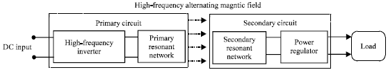 | |
| Fig. 1: | Block diagram of CPT system |
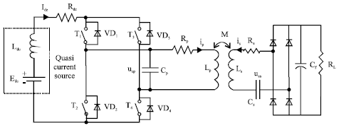 | |
| Fig. 2: | Topology of current-fed CPT system (Edc: DC power supply, Ldc: DC inductor, Rdc: Resistance of Ldc, T1-T4: IGBTs, Cp: Primary capacitor, Lp: Primary inductor, Rp: Resistance of Lp, ip: Current of the primary inductor Lp, M: Mutual inductance, Cs: Secondary capacitor, Ls: Secondary inductor, Rs: Resistance of Ls, is: Current of the secondary inductor Ls, Cf: Filter capacitor, RL: Load resistor) |
The typical topology current-fed CPT system is shown in Fig. 2 which is divided into two parts, primary and secondary.
In the primary side, the input DC voltage source Edc and DC inductor Ldc form a quasi current source. The full-bridge inversion network comprises four switches. Energy transmitter coil Lp and resonant capacitor Cp consist of parallel resonant network, with characteristics like limiting capability, short circuit protection and high reliability. In the secondary side, the energy pickup coil Ls and the resonance capacitor Cs consist of series resonance network, to ensure that the system has received a larger output power.
SYSTEM MODELING BASED ON STROBOSCOPIC MAPPING METHOD
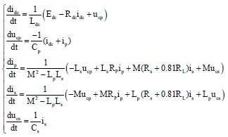
As for multidimensional autonomous nonlinear CPT system, the capacitor voltage and inductor current are taken for state variables in Fig. 2. So x = [idc, ucp, ip, is, ucs]T and input u = [Edc] are state variables of the system and input variables. According to the equivalent circuit model and Kirchhoff's law, each operating cycle of the system can be described by piecewise linearization as differential equation model of two working modes.
Mode 1: Switch (T1, T4) turned on, (T2, T3) turned off, the quasi-current source inject positive energy for resonant network. Steady-state mode lasts for ξ1 = T/2. The mode can be shwon as in Eq. 1:
 | (1) |
Mode 2: Switch (T2, T3) turn on, (T1, T4) turned off, the quasi-current source reversely inject energy for resonant network. Steady-state mode lasts for ξ2 = T/2. The mode can be shown as in Eq. 2:
 | (2) |
So, the state-space description of system is shown in Eq. 3:
| (3) |
Where:
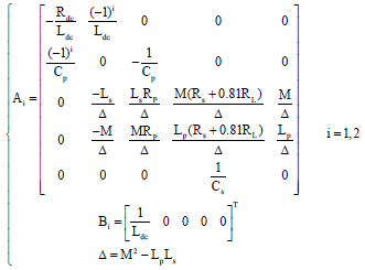 | (4) |
According to the stroboscopic mapping and fixed-point theory modeling method (Tang et al., 2009), the cycle fixed-point function is obtained as in Eq. 5:
| (5) |
Where:
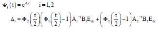 |
Take each component of the cycle fixed-point function x* can obtain the steady-state values of the state variables and thus analyze the operating characteristics of the system.
SYSTEM CHARACTERISTIC MODEL
According to the stroboscopic mapping modeling method and fixed-points theory, a precise mathematical model is established. Each operating frequency and the steady-state values of system state variables under different loads are obtained. Thus soft-switching frequency model of the system, exciting current model, load output voltage model and efficiency of system are obtained to study the system characteristics under different loads.
Soft switching frequency model: The CPT system must work in real-time soft switching state, to reduce switching loss and noise of resonant converter. Therefore, it is necessary to analyze soft-switching frequency characteristics of the system, when load changes. Based on the modeling method above, the primary side capacitor voltage component ucp in the fixed-point functions is taken. Make Yucp = [0, 1, 0, 0, 0], the system fixed-point function is available to analyzes soft-switching resonant frequency and can be expressed as in Eq. 6:
| (6) |
Assume all solutions of the equation fx*(t) = 0 are Ti (i = 1, 2...n). These non-zero solutions are respectively taken as the system switching cycle, so the system has n soft-switching point. As shown in shown in Fig. 2, for the current-fed CPT system, the higher the frequency, the exciting current is reduced and the power transfer capacity becomes weak (Wang et al., 2004). So, the largest soft-switching cycle Tmax is selected to get minimal soft switching frequency as shown in Eq. 7:
| (7) |
The Eq. 7 is shown as soft switching frequency model of the system.
Output voltage model: Steady-state period fixed-point x*(Tmax) can be obtained by the maximum soft-switching period Tmax substituted into the Eq. 11. As this fixed-point is the initial state of the system steady-state period, the piecewise analytic function of each state within steady period can be shown as in Eq. 8:
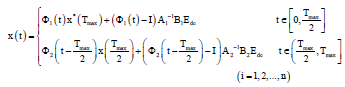 | (8) |
The secondary side resonant current component is in the state functions is taken. Make Yis = [0, 0, 0, 1, 0], so the output voltage uo(t) can be expressed as in Eq. 9:
| (9) |
The Eq. 9 is shown as output voltage model of the system.
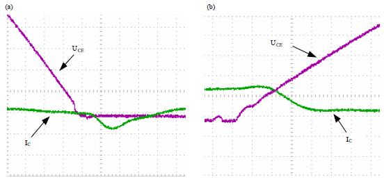 | |
| Fig. 3(a-b): | Waveform of switch, (a) Turn-on and (b) Turn-off |
Exciting current model: Make Yip = [0, 0, 1, 0, 0], so the exciting current ip(t) can be expressed as in Eq. 10:
| (10) |
The Eq. 10 is shown as exciting current model of the system.
Efficiency model: The loss of the system is composed of the inverter loss, copper loss of the coupling mechanism and secondary rectifier is shown in Fig. 2.
Loss model of primary inverter: The primary high-frequency inverter operates at a ZVS condition, so switching loss should be zero under ideal condition. However, there are still some on-state loss and switching loss due to voltage drop and tail current.
| • | Conduction loss: There is a certain on-state voltage drop between the Collector (C) and Emitter (E) when the switch is turned on, so conduction loss of a switch can be calculated in Eq. 11: |
| (11) |
| where Uce and Ic, respectivel represent on-state voltage drop and current of the switch while T is operating cycle | |
| • | Turn-on loss: Due to the bypass diode in IGBT, circulation phenomenon exists in the inverter circuit inevitably (Lv et al., 2012). Such as T1, the tail current results in turn-off delay of a switch. At the switching point, induced electromotive force in the primary inductor Lp form a negative current VD1→T3→Lp→Rp. As shown in Fig. 3a |
So, turn-on loss of a switch can be calculated in Eq. 12:
| (12) |
where, UVD represent bypass diode on-state voltage.
| • | Turn-off loss: As shown in Fig. 3b, the turn-off loss of a switch can be expressed as in Eq. 13: |
| (13) |
| • | Other loss: Other loss of the inverter includes drive loss and copper loss of the DC inductor. Drive loss is caused by the driving voltage charging for the input capacitance Cg, can be expressed as in Eq. 14: |
| (14) |
| where, Cg is the equivalent capacitance of the gate switch, Uge is driving voltage, fs is the switching frequency. |
Copper loss of the DC inductance can be expressed as in Eq. 15:
| (15) |
where, Idc is input current of the inverter, Rdc is internal resistance of the DC inductor.
 | |
| Fig. 4: | Profile of Litz-wire |
The inverter loss during each cycle can be calculated in Eq. 16:
| (16) |
Copper loss model of the coupling mechanism: In order to reduce the impact of skin effect on the system parameters, Litz wire which twisted together by a plurality of thin wires is usually used for winding coupling mechanism. The profile of Litz wire is shown in Fig. 4. Assuming Ns represents the number of wires, Ds is the diameter of a single wire, Dw is the total diameter of the Litz wire.
The relationship between high-frequency AC resistance of Litz-wire and the frequency f of current flowing through the wire is (Sinha et al., 2010):
| (17) |
where, Rdc is DC resistance of Litz-wire, K is AC impedance coefficient which depends on the number of wires Ns.
Thus, copper loss model of the coupling mechanism is shown in Eq. 18:
| (18) |
where Ip and Is, respectively represent rms current of the primary, secondary coil, Rp and Rs, respectively represent high frequency resistance of the primary and secondary coil.
Loss model of secondary rectifier: There are still some conduction loss and switching loss in secondary rectifier.
| • | Conduction loss: The conduction loss of a switch can be calculated in Eq. 19: |
| (19) |
| where, UF and ID, respectively represent conduction voltage and current of the diode | |
| • | Switching loss: Turn-on loss of a diode can be calculated in Eq. 20: |
| (20) |
| where, UFR represents overvoltage of diode, IF represents forward current of diode, trs represents rising time of diode |
| Turn-off loss of a diode can be calculated in Eq. 21: |
| (21) |
where Kf represents reverse recovery temperature coefficient, UR represents backward voltage of diode when turned off, IR represents recovering current of diode, tfs represents recovering time of diode.
The rectifier loss during each cycle can be calculated in Eq. 22:
| (22) |
To get an accurate efficiency model, combined with the loss analysis, system efficiency is determined as in Eq. 23:
| (23) |
According to the mutual model and KVL, KCL equation, the output power Pout, the primary coil power loss PLp, the secondary coil power loss PLs can be respectively, expressed as in Eq. 24 and 25:
| (24) |
| (25) |
where, magnetizing current:
the primary coil resistance: ![]() , the secondary coil resistance:
, the secondary coil resistance: ![]() .
.
Combined Eq. 11-25, efficiency model of the system is obtained.
SIMULATION AND EXPERIMENTAL STUDY
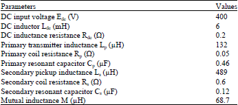
In order to study the characteristic of proposed system intuitionally, the simulation model is built in MATLAB, the parameters are shown in Table 1.
According to Eq. 7 and 10, the waveform of soft switching operating frequency and exciting current with loads vary is plotted in Fig. 5. As the load varies, there is certain constant frequency area and constant current area in the system.
According to Eq. 9, combined the relevant parameters in Table 1, the waveform of output voltage varying with loads can be obtained as shown in Fig. 6.
As can be seen from Fig. 6, when the resonance parameters Cp = 0.46 μF, the output voltage at the load interval [R1, ∞] exists constant region. But in a heavy load(<R1), it does not meet the requirements of constant voltage region. Through changing the value of the resonant capacitor Cp (increased to 0.5 μF), soft-switching frequency of the system is reduced to 19.4 kHz, the constant voltage region can be broadened to [R2, +∞] from [R1, +∞]. Therefore, the resonant frequency can be dynamically adjusted to ensure the system voltage output in a wider range of loads.
According to the system efficiency model, combined the relevant parameters in Table 1, the system efficiency characteristics are shown in Fig. 7. From Fig. 7, as the load changes, there is an optimal frequency to maximize efficiency.
| Table 1: | Parameters of systems |
 | |
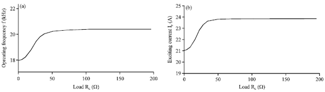 | |
| Fig. 5(a-b): | Curves of primary characteristic varying with loads, (a) Soft switching operating frequency and (b) Exciting current |
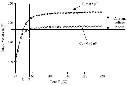 | |
| Fig. 6: | Curves of output voltage varying with loads |
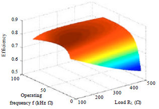 | |
| Fig. 7: | Relationship between efficiency, operating frequency and load |
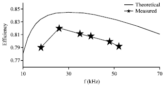 | |
| Fig. 8: | Measured efficiency versus operating frequency f at RL = 100 Ω |
When the system operating frequency is fixed, the system efficiency reduces as the load becomes light. Therefore, when load changes (in particular light load), reasonable optimized frequency contributes to improve system efficiency.
Figure 8 shows the efficiency response versus operating frequency at RL = 100Ω. It can be seen from experiment results that the proposed efficiency model is accuracy. The maximum error of efficiency is 4.2%.
CONCLUSION
Modeling and characteristic analysis of current-fed wireless power transfer system are observed in this study. Loss model of the system is analyzed quantifiably. Through stroboscopic mapping modeling method and fixed points theory, the piecewise linear stroboscopic mapping model of CPT system is established. Soft-switching frequency, output voltage, exciting current and efficiency characteristics when load varies are analyzed based on this model. It can be known that the operating frequency of the system should be controlled to adjust the load changes for ensuring that the system output characteristics remain at a good level.
REFERENCES
- Hu, A.P., J.T. Boys and G.A. Covic, 2000. ZVS frequency analysis of a current-fed resonant converter. Proceedings of the 7th IEEE International Processing of International Power Electronics Congress, October 15-19, 2000, Acapulco, pp: 217-221.
CrossRef - Sun, Y., L. Li, X. Dai, Y. Su and Z. Wang, 2005. Discrete mapping modeling and simulation of a full bridge current-fed soft-switching converter. Trans. China Electrotechnical Soc., 20: 23-27.
Direct Link - Fang, W., H.J. Tang and W. Liu, 2007. Modeling and analyzing an inductive contactless power transfer system for artificial hearts using the generalized state space averaging method. J. Comput. Theor. Nanosci., 4: 1412-1416.
CrossRefDirect Link - Tang, C.S., Y. Sun, Y.G. Su, S.K. Nguang and A.P. Hu, 2009. Determining multiple Steady-state ZCS operating points of a Switch-mode contactless power transfer system. IEEE Trans. Power Electron., 24: 416-425.
CrossRef - Wang, C.S., G.A. Covic and O.H. Stielau, 2004. Power transfer capability and bifurcation phenomena of loosely coupled inductive power transfer systems. IEEE Trans. Ind. Electron., 51: 148-157.
CrossRef - Lv, X., Y. Sun and Z.H. Wang, 2012. Development of current-fed ICPT system with quasi sliding mode control. WSEAS Trans. Cir. Syst., 11: 351-360.
Direct Link