
Sirithip Wasinrat
Department of Statistics, Faculty of Science, Kasetsart University, Bangkhen, Bangkok, 10900, Thailand
Winai Bodhisuwan
Department of Statistics, Faculty of Science, Kasetsart University, Bangkhen, Bangkok, 10900, Thailand
Panlop Zeephongsekul
School of Mathematics and Geospatial, Faculty of Applied Science, RMIT University, Melbourne, VIC 3000, Australia
Ampai Thongtheeraparp
Department of Statistics, Faculty of Science, Kasetsart University, Bangkhen, Bangkok, 10900, Thailand
Journal of Applied Sciences
Year: 2013 | Volume: 13 | Issue: 1 | Page No.: 103-110


ABSTRACT
A traditional approach in the analysis of survival data was assumed a homogeneous population, i.e., all individuals had the same risk of failure or death. For this purpose, the Weibull distribution was very popular, especially in survival analysis. However, most populations consisted of individuals that differed in their susceptibility to causes of death or disease, responses to treatments and influences of various risk factors. This heterogeneity of responses when faced with unexplained factors could cause serious problems when dealt with by traditional methods since it could lead to misleading conclusions. This paper proposed a mixture of two distributions; Weibull hazard rate with a power variance function frailty distribution to model hazard rate. The proposed model included a mixture Weibull hazard rate with gamma and inverse Gaussian distribution. In additional, the parameter estimation for this model via maximum likelihood method was provided. The paper demonstrated its usefulness by applying it to a real data set. The results obtained indicated that the proposed model provided a better fit than the standard Weibull distribution.
PDF Abstract XML References Citation
Received: November 16, 2012;
Accepted: December 31, 2012;
Published: February 01, 2013
How to cite this article
Sirithip Wasinrat, Winai Bodhisuwan, Panlop Zeephongsekul and Ampai Thongtheeraparp, 2013. A Mixture of Weibull Hazard Rate with a Power Variance Function Frailty. Journal of Applied Sciences, 13: 103-110.
DOI: 10.3923/jas.2013.103.110
URL: https://scialert.net/abstract/?doi=jas.2013.103.110
DOI: 10.3923/jas.2013.103.110
URL: https://scialert.net/abstract/?doi=jas.2013.103.110
INTRODUCTION
Survival analysis is a very popular tool in analyzing failure data such as death of biological organisms or failure of mechanical systems. It plays an important role in medicine, epidemiology, biology and demography. In engineering, it is often referred to as reliability analysis. A standard approach in survival analysis is to assume that the population is homogeneous, that is, every individual has the same risk of death or failure. For this purpose, the Weibull distribution has been used extensively to analyze survival data. As is well known, the Weibull distribution generalizes the exponential distribution since it can incorporate increasing, decreasing and constant hazard rates (Lee and Wang, 2003) whereas, the hazard rate of the exponential distribution is constant. Some recent examples of the application of the Weibull distribution to survival analysis can be found by Mudholkar et al. (1996) and Saat and Jemain (2009). Many authors have proposed new distributions based on the traditional Weibull distribution (Pham and Lai, 2007).
The assumption of a homogeneous population in most literature on survival analysis is not always realistic (Vaupel et al., 1979; Hougaard, 1984, 2000). In general, the population consists of individuals that differ in their susceptibility to causes of death or failure, responses to treatments and influences of various risk factors. Furthermore, it is not always possible to include all risk factors or covariates into the model. In addition, there are always unknown and unobservable risk factors which can cause further heterogeneity within the population. To overcome these problems, a random variable incorporating these unknown or unobservable risk factors is included in the models for analysis of survival data. This random variable, known as frailty, was introduced by Vaupel et al. (1979) and acts multiplicatively on the hazard function. The resulting modified hazard model, where the frailty variable is multiplied by the baseline hazard function, is called a frailty model (Hougaard, 1984; Aalen, 1988).
The underlying distribution most often used in association with the frailty model is the gamma distribution due to its mathematical tractability. Other choices are the inverse Gaussian (Hougaard, 1986; Keiding et al., 1997; Kheiri et al., 2007) and the positive stable distribution (Qiou et al., 1999). An extended family of frailty distribution called the Power Variance Function (PVF), which includes the gamma, inverse Gaussian and positive stable distribution as special cases, was introduced by Hougaard (1986). Subsequently, the PVF distribution was reparameterized by Aalen (1992) and applied under various contexts by Hanagal (2008, 2009). The distribution provided additional flexibility when applying frailty models to real data.
In this study, we introduce the mixed Weibull hazard function with the frailty term and PVF distribution to accommodate the problem of a heterogeneous population. Since the proposed model includes four unknown parameters, we discuss the use of Maximum Likelihood Estimation (MLE) for estimating these parameters. Finally, the proposed model is applied to a real data set involving sufferers of AIDS (Acquired Immunodeficiency Syndrome) to evaluate its usefulness.
A MIXTURE WEIBULL HAZARD RATE WITH PVF FRAILTY
Let T be an arbitrary continuous nonnegative random variable and Z be an nonnegative random variable, called the frailty or mixing random variable. The frailty model is the product of a random effect Z and baseline hazard rate. The conditional hazard rate and survival function, respectively are:
h(t|Z) = Zh0(t) |
and
S(t|Z) = e-ZH0(t) |
where, h0(t) is called baseline hazard function and ![]() is the cumulative baseline hazard function (Vaupel et al., 1979).
is the cumulative baseline hazard function (Vaupel et al., 1979).
If Z be a frailty random variable with probability density function (pdf) f(z) then the marginal survival function or mixture survival function can be derived by using the Laplace transform of Z (Hougaard, 2000). The marginal survival function or mixture survival function, denoted SM(t) is given by:
SM(t) = [e-ZH0(t)] = LZ[H0(t)] |
Where:
is the Laplace transform of Z. The mixture hazard rate, denoted hM(t) is given by:
Weibull distribution: Let T be a random variable distributed as Weibull distribution with parameters η and γ then the pdf denoted by Weibull (η, γ) is given by:
| (1) |
The survival function of the Weibull distribution is:
| (2) |
The corresponding hazard function and cumulative hazard function, respectively are:
| (3) |
and
| (4) |
PVF frailty distribution: Let Z be non-negative frailty random variable from the PVF distribution. The pdf of Z is given by:
where, μ>0, δ>0 and 0<v<1 (Aalen, 1992; Duchateau and Janssen, 2008). The corresponding Laplace transform is:
where, E(Z) = μ and Var(Z) = δμ2 are mean and variance, respectively. In order to avoid an unidentifiable scale factor, in the frailty model, it is common practice to take the mean of the frailty distribution as equal to 1. If the parameter μ = 1 then E(Z) = 1 and Var(Z) = δ. The Laplace transform under the mean equal to 1 is:
| (5) |
with δ = 0 and 0<v<1.
Under baseline cumulative hazard function in Eq. 4 and the Laplace transform in Eq. 5, we can obtain the marginal survival of the mixture Weibull with the PVF distribution:
| (6) |
and the corresponding mixture hazard function is:
| (7) |
where, η>0, γ>0, δ>0 and 0<v<1.
Theorem 1: Let T be a random variable of the mixture Weibull hazard rate with PVF frailty distribution, denoted by T~Weibull-PVF (η, γ, δ and v). The pdf of T is given by:
where, η>0, γ>0, δ>0 and 0<v<1.
Proof: Since:
| (8) |
We substitute hM(t) in Eq. 8 with 7 and SM(t) in Eq. 8 with 6, we obtain:
with η>0, γ>0, δ>0 and 0<v<1.
The pdf plot of some values of the parameters is shown in Fig. 1 and its survival function and hazard function are presented, respectively in Fig. 2 and 3.
The Weibull-PVF distribution includes some mixture hazard function, i.e.:
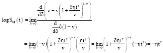
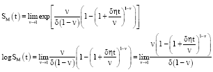
| • | If v = 1/2 then the Weibull-PVF can be reduced to the mixture Weibull hazard rate with the inverse Gaussian frailty distribution (Weibull-Gamma) which its hazard function given by: |
| (9) |
and the survival function associated with Eq. 9 is:
This is related to the inverse Gaussian frailty distribution (Duchateau and Janssen, 2008).
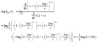
| • | If v = 1 then the Weibull-PVF can be reduced to the mixture Weibull hazard rate with the gamma frailty distribution (Weibull-IG) which its hazard function given by: |
| (10) |
and the survival function associated with Eq. 10 is:
SM(t) = [1+δηtγ]-(1/δ) |
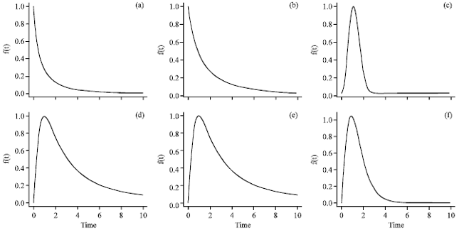 | |
| Fig. 1(a-f): | The pdf plots of Weibull-PVF (η, γ, δ, v) (a) 1, 1, 1, 0.5, (b) 0.5, 1, 1, 0.5, (c) 0.5, 3, 0.5, 0.2, (d) 2, 2, 3, 0.7 (e) 1, 2, 1, 0.9 and (f) 0.5, 2, 0.5, 0.5, f(t): Probability density function |
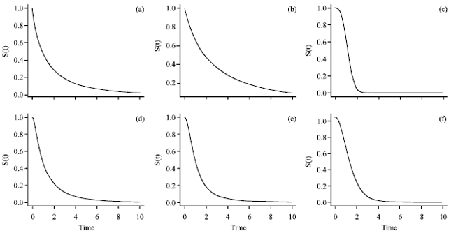 | |
| Fig. 2(a-f): | Some plots of Weibull-PVF (η, γ, δ, v) (a) 1, 1, 1, 0.5, (b) 0.5, 1, 1, 0.5, (c) 0.5, 3, 0.5, 0.2, (d) 2, 2, 3, 0.7, (e) 1, 2, 1, 0.9 and (f) 0.5, 2, 0.5, 0.5, S(t): Survival function |
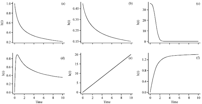 | |
| Fig. 3(a-f): | The hazard shapes under Weibull-PVF (η, γ, δ, v) (a) 1, 1, 1, 0.5, (b) 0.5, 1, 1, 0.5, (c) 0.5, 3, 0.5, 0.2, (d) 2, 2, 3, 0.7, (e) 1, 2, 1, 0.9 and (f) 0.5, 2, 0.5, 0.5, h(t): Hazard function |
It is the Weibull-Gamma frailty model (Molenberghs and Verbeke, 2011).
Moreover, the Weibull-PVF distribution is also related to well known distributions, e.g., Weibull and Lomax distribution as shown in the following Corollary 1 and 2.
Corollary 1: If δ→0, δ>0 then the Weibull-PVF (η, γ, δ, v) distribution reduces to the Weibull (η, γ).
Proof: First, we consider the hazard function of Weibull-PVF (η, γ, δ, v) if δ→0, δ>0, then:
| (11) |
Which is equivalent to Eq. 3. The survival function of Weibull-PVF (η, γ, δ, v) when δ→0, δ>0 can be derived as follows:
 |
Since the limit leads to 0/0, we then apply the L’Hospital’s rule:
 |
Hence:
| (12) |
Consequently, we will obtain the pdf of Weibull-PVF (η, γ, δ, v) when δ→0 based on Eq. 11 and 12 is:
fM(t) = hM(t).SM(t) = ηγtγ-1 exp(-ηtγ) |
Corollary 2: If v→1, 0<v<1 and γ is equal to 1 then the Weibull-PVF (η, γ, δ, v) distribution reduces to the Lomax distribution (Lomax, 1954), also called the Pareto type II distribution with parameters ![]() which pdf given by:
which pdf given by:
Proof: By substituting v = 1 and γ = 1 in Eq. 7, we obtain:
| (13) |
and the survival function in Eq. 6, if v→1 and γ = 1, then:
 |
Since the limit leads to 0/0, we then apply the L’Hospital’s rule:
 |
Therefore:
| (14) |
We then obtain the pdf of the Lomax distribution as:
ESTIMATION OF PARAMETERS
The MLE is the most popular method of estimation and inference for parametric models. Recall that, if t1, t2,…, tn are random samples from a population with a pdf ![]() where
where ![]() is a vector of parameters, then the likelihood function is defined by:
is a vector of parameters, then the likelihood function is defined by:
The likelihood function for the Weibull-PVF distribution where ![]() , can be written as:
, can be written as:
 |
and let L (·) = log L (·) which is in the form:
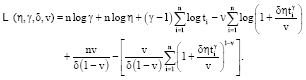 |
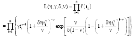
In real life problem of survival data analysis, we often found with the right censored data. This paper derives the likelihood function and the log-likelihood function for the Weibull-PVF distribution under right censored data.
The likelihood function for right censored data is defined as:
where, di is the censoring indicator, taking the value one if the event is occurred, otherwise di take value zero. The log likelihood function for the Weibull-PVF distribution with right censored data where ![]() , can be written as:
, can be written as:
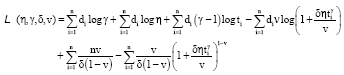 |
We can find the MLE by using a numerical method to optimize the equation:
Since the first derivatives of the log likelihood function are so complicated and it is hardly to solve this system of equations. We then use the Newton-Raphson procedure as the alternate iterative algorithm for estimating the parameters under MLE.
APPLICATION TO AIDS DATA SET
Selvin (2008) presented data from the San Francisco Men’s Health Study (SFMHS) which was conducted in 1983 as a population-based study of the epidemiology and natural history of the newly emerging AIDS. The data explored here are a small subset consisting of the 174 individuals who entered the study during the first year. Survival time is defined as the number of months from diagnosis of AIDS to death with right censoring. In this study we omit the covariates.
We fit the AIDS data set under the Weibull, Weibull-Gamma, Weibull-IG and Weibull-PVF. The results of the estimated parameters by using MLE and the log-likelihood values are shown in Table 1. This study utilizes the survival function obtained by using the Kaplan-Meier estimate. The obtained survival curves based on Weibull, Weibull-Gamma, Weibull-IG and Weibull-PVF are in Fig. 4. Moreover, the histograms of the AIDS data with fitted curves of Weibull, Weibull-Gamma, Weibull-IG and Weibull-PVF are shown in Fig. 5.
The log-likelihood value of Weibull-PVF is-632.2820, which is better than that of Weibull, Weibull-Gamma and Weibull-IG.
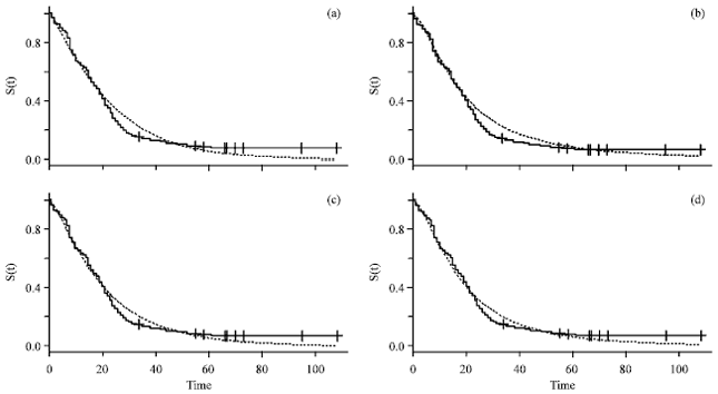 | |
| Fig. 4(a-d): | The estimated survival curves using Kaplan-Meier based on (a) Weibull, (b) Weibull-Gamma, (c) Weibull-IG and (d) Weibull-PVF model, S(t): Survival function |
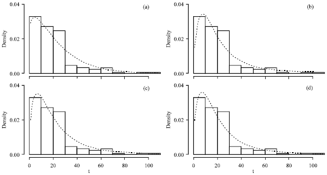 | |
| Fig. 5(a-d): | The histograms of the AIDS data with fitted (a) Weibull, (b) Weibull-Gamma, (c) Weibull-IG and (d) Weibull-PVF model |
| Table 1: | Estimated parameters and log-likelihood values of different models for the AIDS data set |
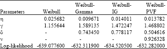 | |
That is, the Weibull-PVF model is more effectively fit to this data set than Weibull, Weibull-Gamma and Weibull-IG which are shown Fig. 4 and 5.
In addition, the log-likelihood values which are shown that the mixture Weibull model provides a better fit compare to the standard Weibull model for this data set when omits covariates or risk factors. However, the Weibull-PVF is more flexible than Weibull Gamma and Weibull-IG since it includes the both models as a special cases.
CONCLUSION
In this study, we introduced the four-parameters Weibull-PVF distribution. This model included Weibull-Gamma and Weibull-IG as sub-models and related to Weibull and Lomax distribution. Figure 1-3 showed the pdf plots, survival curves and hazard shape of Weibull-PVF for some values of parameter, respectively. The MLE was used to estimate model parameters. It was also included the likelihood function for right censored data, which often occurs in survival analysis. Furthermore, the AIDS data with right censoring from the SFMHS is applied to model fitting. The data was fitted to the Weibull, Weibull-Gamma, Weibull-IG and Weibull-PVF models, we found that the Weibull-PVF model gave the best fit. Thus, we can say that the Weibull-PVF distribution is an alternative model for heterogeneous populations in survival analysis.
ACKNOWLEDGMENTS
We are grateful to the Commission on Higher Education, Thailand, for financial support through a grant fund under the Strategic Scholarships Fellowships Frontier Research Networks.
REFERENCES
- Aalen, O.O., 1992. Modelling heterogeneity in survival analysis by the compound Poisson distribution. Ann. Applied Probab., 2: 951-972.
Direct Link - Hanagal, D.D., 2009. Modeling heterogeneity for bivariate survival data by power variance function distribution. J. Reliab. Stat. Stud., 2: 14-27.
Direct Link - Hanagal, D.D., 2008. Frailty regression models in mixture distributions. J. Stat. Plann. Inference, 138: 2462-2468.
CrossRef - Hougaard, P., 1984. Life table methods for heterogeneous populations: Distributions describing the heterogeneity. Biometrika, 71: 75-83.
CrossRef - Hougaard, P., 1986. Survival models for heterogeneous populations derived from stable distributions. Biometrika, 73: 387-396.
Direct Link - Kheiri, S., A. Kimber and M.R. Meshkani, 2007. Bayesian analysis of an inverse Gaussian correlated frailty model. Comput. Stat. Data Anal., 15: 5317-5326.
CrossRef - Lomax, K.S., 1954. Business failures: Another example of the analysis of failure data. J. Am. Stat. Assoc., 49: 847-852.
Direct Link - Molenberghs, G. and G. Verbeke, 2011. On the Weibull-Gamma frailty model, its infinite moments and its connection to generalized log-logistic, logistic, Cauchy and extreme-value distributions. J. Stat. Plann. Inference, 141: 861-868.
CrossRef - Mudholkar, G.S., D.K. Srivastava and G.D. Kollia, 1996. A generalization of the Weibull distribution with application to the analysis of survival data. J. Am. Stat. Assoc., 91: 1575-1583.
Direct Link - Pham, H. and C.D. Lai, 2007. On recent generalizations of the Weibull distribution. IEEE Trans. Reliab., 56: 454-458.
CrossRef - Qiou, Z., N. Ravishanker and D.K. Dey, 1999. Multivariate survival analysis with positive stable frailties. Biometrics, 55: 637-644.
PubMed - Saat, N.Z.M. and A.A. Jemain, 2009. Modelling the duration of hypopnea. J. Applied Sci., 9: 2162-2167.
CrossRefDirect Link - Vaupel, J.W., K.G. Manton and E. Stallard, 1979. The impact of heterogeneity in individual frailty on the dynamics of mortality. Demography, 16: 439-454.
CrossRefPubMedDirect Link