
Windarta
Department of Mechanical Engineering, Universiti Teknologi PETRONAS, Bandar Seri Iskandar, 31750 Tronoh, Perak, Malaysia
M. Bin Sudin
Department of Mechanical Engineering, Universiti Teknologi PETRONAS, Bandar Seri Iskandar, 31750 Tronoh, Perak, Malaysia
M.B. Baharom
Department of Mechanical Engineering, Universiti Teknologi PETRONAS, Bandar Seri Iskandar, 31750 Tronoh, Perak, Malaysia
Journal of Applied Sciences
Year: 2012 | Volume: 12 | Issue: 23 | Page No.: 2424-2429


ABSTRACT
The interaction between rail and wheel materials produce wear damage on each surface and frictional heat. This study is aimed to predict contact temperature due to the interaction between rail and wheel for various applied load and velocity. The frictional heat was modeled as a solid contact pressure. The temperature rise was calculated by numerically integrating the equation using Adomian Decomposition Method. The paper also studies the influences of sliding speed on temperature rise. The pin-on-disc experiment was used to validate the results. The results show the peak pressure distributions increase linearly with the increasing applied load with an average slope of 0.053. The maximum temperature rise was 259.98 K at x = 1 mm for 5.3 MPa pressure and 3.14 m sec-1 sliding speed. Prediction temperature rise results were successfully validated using pin-on-disc method. The average error between prediction and measurement results was 4.99 %.
PDF Abstract XML References Citation
Received: September 01, 2012;
Accepted: November 05, 2012;
Published: January 02, 2013
How to cite this article
Windarta, M. Bin Sudin and M.B. Baharom, 2012. Prediction of Contact Temperature on Interaction between Rail and Wheel Materials Using Pin-on-Disc Method. Journal of Applied Sciences, 12: 2424-2429.
DOI: 10.3923/jas.2012.2424.2429
URL: https://scialert.net/abstract/?doi=jas.2012.2424.2429
DOI: 10.3923/jas.2012.2424.2429
URL: https://scialert.net/abstract/?doi=jas.2012.2424.2429
INTRODUCTION
The contact temperature distribution at the interface of rail and wheel materials has been a topic for along time tribology research. Contact temperature distribution is critical for thermal stress analysis between two sliding bodies (Johnson and Greenwood, 1997; Chen and Wang, 2008) and thermal wear modeling (Bucher et al., 2006; Fischer et al., 1997). Contact temperature may influence material properties (Habeeb et al., 2008). Heat is generated due to frictional heating when a body slides on another body. The heat generated between two contact bodies is influenced of the thermal properties of the bodies, the contact geometry and the sliding speed.
One of the first models for estimating contact temperature was proposed by Blok (1963). The maximum temperature rises at the interface of two bodies are the same. The maximum temperature is independent of the speed at low Peclet numbers. The maximum temperature rise at the interface was calculated using a stationary heat source. Similar with Blok (1963) analysis, Carslaw and Jaeger (1938) and Gallardo-Hernandez et al. (2006) presented an analytical integral formula for the temperature rise on the halfspace surface. However, their method was based on the average temperature rise instead of the maximum temperature rise.
The main objective of this study is to determine contact temperature on interaction between rail and wheel materials for various applied load and sliding velocity. The present model is based on pin-on-disc method. The model was applied to simulate the sliding contact of a half-space wheel material over a stationary sphere rail material. Results of pressure and contact temperature under different sliding speeds and applied load were discussed and compared.
MATERIALS AND METHODS
Contact problem: There are two kinds of mechanism contacts between rail and wheel (Fig. 1). First existing one is rolling-sliding contact which occurs on railhead and wheels tread contact. The second is pure sliding contact which occurs on rail edge and wheel flange. In this study, the contact between rail and wheel can be assumed as non conformal contact.
 | |
| Fig. 1: | Overview of wheel-rail contacts |
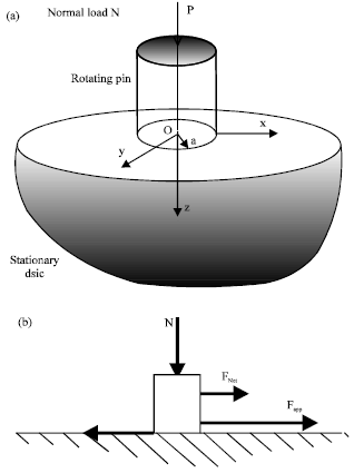 | |
| Fig. 2(a-b): | Pin-on-disc scheme |
A non conformal contact of two bodies in revolution is classified in the general elastic contact. Depending on their modulus of elasticity, the two bodies will deform to certain degrees. The problem may be reduced to that of a single equivalent elastic body revolution on a plain infinitely rigid body. This assumption is widely adopted in the theory and application of Hertzian contacts so that the conversion formulas of geometry and elasticity are well established (Al-Bender and De Moerlooze, 2008; Enblom and Berg, 2008).
When at the top of an elastic pin of radius r and equivalent modulus of elasticity Ee (Fig. 2) is pressed with a load N against a rigid plane disc surface, there is a mark on the contact area (Knothe and Liebelt, 1995; Olofsson and Telliskivi, 2003; Sundh and Olofsson, 2011). The equivalent modulus elasticity is given by:
| (1) |
The pin is rotating with a fixed angular speed ω. Due to the normal force, angular velocity and coefficient of friction μ, a reaction force will occur. This reaction force is frictional force Ff:
| (2) |
| Table 1: | Nominal chemical composition of the studied steel |
| (3) |
The net force FNet is equal applied force Fapp minus frictional force Ff Eq. 3. The contact patch is defined as the region A in the xy-plane: A = {(x, y): x2+y2 = r2}.
The normal stress Pz is given by (Al-Bender and De Moerlooze, 2008):
| (4) |
The magnitude of these axes depends on the radii and the radii of curvature of the contacting systems and on the normal load.
Since, the maximum heat flux occurs in the z direction, the problem can be simplified into two dimensional contacts. The maximum pressure for this case is (Jendel, 2002):
| (5) |
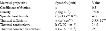
The materials used in this research are rail steels. The chemical composition of material is shown in Table 1.
Pin-on-disc is commonly used in wear test. The tests use Ducom multi specimen testing machine designed according to ASTM G99 standards. Rail steel was cut to form disc specimen which is 42 mm in diameter and 5 mm in width. Pin samples were prepared as 6 mm in diameter and 12 mm in length. During wear tests, the normal forces were applied. The normal force of 40 N, 60 N, 80 N and 100 N were selected. Both pin and disc sample were polished using 120, 220 and 500 grit abrasive papers and cleaned with alcohol and dried.
Heat transfer equations: The assumption is introduced an energy equation problem to determine the temperature field in the wheel-rail contact. The energy equation heat transfer equation will be governed based on Fig. 2:
| (6) |
If the density of a solid is constant, cp = cv. Dividing Eq. 6 by k and replacing k/ρcp by α, the thermal diffusivity of the material:
| (7) |
The differential equation that governs the steady state temperature field is:
| (8) |
Mazidi et al. (2011) proposed that there is a heat partition at the contact surface of two sliding components, because of thermal resistance due to accumulation wear particles. If the frictional heat is the only internal heat generation source (Ertz and Knothe, 2002), then:
| (9) |
| Where | ||
| v | = | Sliding velocity and within the contact area heat is generated owing to friction. The following assumptions were made: |
| • | There is pure sliding within the whole contact area |
| • | The effects of elastic deformation are negligible. Consequently, the local relative velocity equals the global sliding velocity vs |
| • | The heat flow rate q (i.e., the product of the friction coefficient μ, the normal pressure P(x) and the sliding velocity) is transformed completely into heat |
Temperature prediction of pin and disc: The schematic diagram of the temperature at some point (r, θ, z, t) within a pin cylinder of length 2L and radius R, is shown in Fig. 2. The cylinder initially at temperature Ta, at time zero, it is exposed to a fluid at temperature T∞, with convection coefficient of h, Temperature within the cylinder is a function of (r, θ, z, t), for a system with internal heat generation:
| (10) |
The differential equation can be solved by the Adomian Decomposition method, with the assumption of coefficient of friction is constant. Solution for the temperature of any point located at the position (r, θ, z, t) of a cylinder at any time t is T = T (r, θ, z, t) and k is thermal diffusivity. Equation 10 can be rewrite in an operator form by:
| (11) |
where, the differential operators Lr, Lθ and Lz are defined by (Wazwaz, 2002):
| (12) |
So that the integral operator Lt-1 exist and given by:
| (13) |
Applying Lt-1 to both sides of Eq. 13 and using the initial condition lead to:
 | (14) |
The decomposition method defines the solution T (r, θ, z, t) as a series given by:
| (15) |
Substituting Eq. 14 into both sides of Eq. 15 yields:
 | (16) |
The components Tn (r, θ, z, t), n≥0 can be completely determined by using the recursive relationship:
| (17) |
 | (18) |
Where:
| (19) |
RESULTS AND DISCUSSION
Figure 3 shows comparisons of pressure distribution for various applied load. The pressure distribution is calculated based on Hertzian contact solutions. Pressure distribution obtained from the purely elastic analysis well matches that of the analytical Hertz solution.
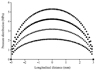 | |
| Fig. 3: | Pressure distribution for various applied load |
| Table 2: | Contact parameters and material properties |
 | |
The peak pressure distribution occurs at the centre of contact, x = 0. The peak pressure distributions increase linearly with the increasing applied load with an average slope of 0.053. These results are same trend with Windarta et al. (2011) conclusions. The pressure and wear rate increase linearly with increasing applied load.
However, the temperature rise due to frictional heating softens the material (degrades the yield strength) when the thermal softening effect is included which further decreases the von Mises stress intensity. Table 2 contains the circular contact parameters and material properties for temperature calculation throughout this study.
Figure 4 presents the comparison of contact temperature profiles along the x axis for various models. Chen and Wang (2008) Model assumes purely elastic contact based on Hertzian contact. There is not any temperature rise outside contact area. The contact pressure is approximately symmetric with respect to x = 0. Ertz and Knothe (2002) proposes a model using four degree polynomial. However, frictional heating distorts the contact pressure distribution under higher sliding speeds and shifts the pressure profile along the mating surface sliding direction. Proposed model modified (Ertz and Knothe, 2002) model, using assumption that frictional heating outside contact produce by conduction and fixed source from contact area.
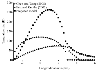 | |
| Fig. 4: | Contact temperature rise comparison along the longitudinal (x) axis with respect to various models |
 | |
| Fig. 5: | Peak temperatures rise with respect to sliding velocity |
The maximum temperature rise is 259.98 K at x = 1 mm for 5.3 MPa pressure and 3.14 m sec-1 sliding speed. The peak temperatures rise with respect to sliding velocity present in Fig. 5.
The surface temperature rise model developed is evaluated based on a pure sliding circular Hertzian contact between an adiabatic moving surface and a stationary surface is considered. In this case, all of the frictional heat is transferred into the stationary surface.
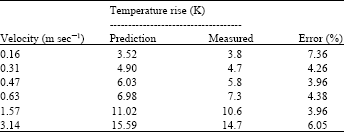
Comparisons between prediction temperature rise and pin-on-disc measurement results with respect to sliding velocity are presented in Table 3. The measurement were taken 6 mm from the centre of pin and disc contact. Average error between prediction and measurement results is 4.99%. The highest error occurs at low sliding velocity (0.16 m sec-1).
Figure 6 gives the variation of the surface temperature rise distribution along the x-axis with respect to the increasing sliding speed.
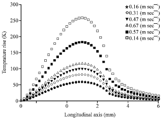 | |
| Fig. 6: | Distributions of surface temperature rise along the x axis corresponding to various sliding velocities |
| Table 3: | Temperature rise comparison for various sliding speed |
 | |
The surface temperature rise increases noticeably as the sliding speed increases (the maximum temperature increases by about 500% when the sliding speed changes from 0.16-3.14 m sec-1. The temperature rise distribution becomes skew under higher sliding speeds (the maximum temperature shifts from the center to the leading edge of the contact area). This trend of temperature with the sliding speed is consistent with that by Chen and Wang (2008).
CONCLUSION
The pressure distribution is calculated based on Hertzian contact solutions. Pressure distribution obtained from the purely elastic analysis well matches that of the analytical Hertz solution. The peak pressure distributions increase linearly with the increasing applied load with an average slope of 0.053.
The maximum temperature rise is 259.98 K at x = 1 mm for 5.3 MPa pressure and 3.14 m sec-1 sliding speed. Prediction temperature rise results were successfully validated using pin-on-disc method. Average error between prediction and measurement results is 4.99%. The highest error occurs at low sliding velocity (0.16 m sec-1).
ACKNOWLEDGMENT
The authors would like to thank Keretapi Tanah Melayu Berhad (KTMB) for providing railway and wheel materials. This research is under Graduate Assistantship Universiti Teknologi PETRONAS.
NOMENCLATURE
| a0, p0 | = | Hertz contact radius (mm) and peak pressure (MPa) |
| Ei | = | Young’s modulus two contact bodies (i = 1 and 2) |
| E* | = | Equivalent Young’s modulus (GPa) |
| H | = | Hardness (GPa) |
| k | = | Thermal conductivity (W m-1 K-1) |
| l | = | Characteristic length (mm) |
| p, s | = | Pressure and shear traction (MPa) |
| q, q1, q2 | = | Total heat flux and heat flux flowing to two bodies (W m-2 ) |
| ΔT | = | Temperature rise (K) |
| Tm, Ta | = | Material melting point and reference room temperature (K) |
| Vs | = | Sliding velocity (m sec-1) |
| W | = | Normal load (N) |
| x, y, z | = | Space coordinates (mm) |
| α | = | Linier thermal expansion coefficient (mm K-1 m-1) |
| δ | = | Rigid body approach (mm) |
| Δ | = | Mesh size (mm) |
| μf | = | Coefficient of friction |
| υi | = | Poisson ratio of two contact bodies |
| σij | = | Total stress component (MPa) |
| σVM | = | Von Mises equivalent stress (MPa) |
| σy | = | Initial yield strength (MPa) |
REFERENCES
- Al-Bender, F. and K. De Moerlooze, 2008. A model of the transient behavior of tractive rolling contacts. Adv. Tribol., Vol. 2008.
CrossRef - Bucher, F., A.I. Dmitriev, M. Ertz, K. Knothe, V.L. Popov, S.G. Psakhie and E.V. Shilko, 2006. Multiscale simulation of dry friction in wheel/rail contact. Wear, 261: 874-884.
CrossRef - Carslaw, H.S. and J.C. Jaeger, 1938. On green's functions in the theory of heat conduction. Philos. Mag., 26: 473-495.
Direct Link - Chen, W.W. and Q.J. Wang, 2008. Thermomechanical analysis of elastoplastic bodies in a sliding spherical contact and the effects of sliding speed, heat partition and thermal softening. J. Tribol., Vol. 130.
CrossRef - Enblom, R. and M. Berg, 2008. Proposed procedure and trial simulation of rail profile evolution due to uniform wear. Proc. Inst. Mech. Eng. F, J. Rail Rapid Transit, 222: 15-25.
CrossRef - Ertz, M. and K. Knothe, 2002. A comparison of analytical and numerical methods for the calculation of temperatures in wheel/rail contact. Wear, 253: 498-508.
CrossRef - Fischer, F.D., E. Werner and W.Y. Yan, 1997. Thermal stresses for frictional contact in wheel-rail systems. Wear. 211: 156-163.
CrossRef - Gallardo-Hernandez, E.A., R. Lewis and R.S. Dwyer-Joyce, 2006. Temperature in a twin-disc wheel/rail contact simulation. Tribol. Int., 39: 1653-1663.
CrossRef - Habeeb, H.H., K.A. Abou-El-Hossein, B. Mohamad, J.A. Ghani and K. Kadirgama, 2008. Investigating of tool wear, tool life and surface roughness when machining of nickel alloy 242 with using of different cutting tools. Asian J. Scientific Res., 1: 222-230.
CrossRefDirect Link - Jendel, T., 2002. Prediction of wheel profile wear-comparisons with field measurements. Wear, 253: 89-99.
CrossRef - Johnson, K.L. and J.A. Greenwood, 1997. An adhesion map for the contact of elastic spheres. J. Colloid Interface Sci., 192: 326-333.
CrossRef - Knothe, K. and S. Liebelt, 1995. Determination of temperatures for sliding contact with applications for wheel-rail systems. Wear, 189: 91-99.
CrossRef - Mazidi, H., S. Jalalifar, S. Jalalifar and J. Chakhoo, 2011. Mathematical modeling of heat conduction in a disk brake system during braking. Asian J. Applied Sci., 4: 119-136.
CrossRefDirect Link - Olofsson, U. and T. Telliskivi, 2003. Wear, plastic deformation and friction of two rail steels-a full-scale test and a laboratory study. Wear, 254: 80-93.
CrossRef - Sundh, J. and U. Olofsson, 2011. Relating contact temperature and wear transitions in a wheel-rail contact. Wear, 271: 78-85.
CrossRef - Windarta, M.B. Sudin and K. Fuad, 2011. Influence of applied load on wear characterizations of rail material. J. Applied Sci., 11: 1636-1641.
CrossRef