
E. Nissi
Dipartimento di Metodi Quantitativi e Teoria Economica, Viale Pindaro, 42 -65127, Pescara
A. Sarra
Dipartimento di Metodi Quantitativi e Teoria Economica, Viale Pindaro, 42 -65127, Pescara
Journal of Applied Sciences
Year: 2011 | Volume: 11 | Issue: 4 | Page No.: 630-638


ABSTRACT
The development of local forms of spatial analysis has been the subject of intense research over last decade. The condition that observations are independent is not frequent in spatial data analysis. Parameter drift is often recognized when a model is calibrated separately across locations in space. In this study, we propose a local calibration procedure for handling varying parameters estimates of an origin-constrained spatial interaction model. In this context, the estimates of local parameters depend both on origins and destinations and a four dimensional space is involved. A suite of local parameters can be obtained by the maximisation of a weighted maximum likelihood function, exploiting the same principle of Geographically Weighted Regression (GWR) approach. Generally, the function for the weighting scheme in GWR uses only distance (geographical space) to determine weights. We propose a modified version of weighting function which takes into account both the spatial distance and a function of strength of connection between two specific destinations. The performance of different weighting functions for modelling the effects of spatial heterogeneity on flow data are compared and evaluated.
PDF Abstract XML References Citation
Received: October 16, 2010;
Accepted: November 13, 2010;
Published: February 12, 2011
How to cite this article
E. Nissi and A. Sarra, 2011. Detecting Local Variations in Spatial Interaction Models by Means of Geographically Weighted Regression. Journal of Applied Sciences, 11: 630-638.
DOI: 10.3923/jas.2011.630.638
URL: https://scialert.net/abstract/?doi=jas.2011.630.638
DOI: 10.3923/jas.2011.630.638
URL: https://scialert.net/abstract/?doi=jas.2011.630.638
INTRODUCTION
Spatial interaction models focus on origin-destination pairs of regions and use flow data. They have been applied in many contexts in order to understand and explain movements of people, commodities, information, ideas, capital or knowledge from one set of places to another (migration studies, shopping, travel to work, airline passengers traffic). The simplest form of spatial interaction models is based on the analogy of Newton’s law of gravity in physics. Basically, the flow between two places is a function of the ability of an origin to generate flows (the so-called propulsiveness), the capability of a destination to attract flows (the so-called attractiveness) and a sensible measure of separation of origin and destination (typically named spatial impedance). More solid foundations to spatial interaction models was provided by A.G. Wilson by their statistical mechanics entropy formulation, which ensures that these models can be cast in a probabilistic form (Roy, 2004). Traditionally, fitting the spatial interaction models to the observed data, is a question of estimating the unknown parameters: the ones characterising the propensity of each origin to generate flows, the ones characterising the attractiveness of each destination and the one related to distance deterrence effect. One way to enhance the spatial interaction modelling is to properly take into account the parameters instability across the space, otherwise it would be possible to discover a severe misspecification bias in the general spatial interaction modelling formula (Tiefelsdorf, 2003). For example, if the distance decay parameter is not stable across the space, we can observe a counter-intuitive finding: an amplification of interaction as distance increases. Model parameters can be correctly interpreted only once spatial structure effects are under control. According to Fotheringham (1981), spatial structure can be defined as the size and configuration of the origins and destinations of regional system under investigation. The underlying spatial structure of spatial interaction models can be tackled from different points of view. Fotheringham (1983) proposes to introduce in the modelling a Competing Factor (CD) which represents the relationship between destination j and all other destinations, also named accessibility variable. The essential idea is that the movers are faced with a set of destinations competing for their attention: the more accessible a destination is to all other destinations in a spatial system, the less likely it is that destination is a terminating point for interaction from any given origin, ceteris paribus. The spatial proximity perspective expects competition only by spatial association. Lately, Jim (1998) proposes an alternative viewpoint on competition among destinations, which contemplates the idea that destinations which are widely separated in space, or which vary greatly in size and/or distance from a given origin, may exert nevertheless identical influences on decision makers at that origin. Anyway, competing destinations models represent a good example for identifying of the misspecification global models and for improving the global statements of spatial behaviour. Another approach which attempts to accommodate spatial heterogeneity, by allowing the parameters of the model to vary with the spatial location of data, regards the expansion method of Casetti (1972) and Jones and Casetti (1992). Recently, Fischer and Griffith (2008) illustrate two approaches for a proper specification of spatial interaction models, facing with the problem of accounting for spatial autocorrelation effects. Firstly, following a spatial econometric perspective, they specify a spatial process for the disturbance terms reflecting origin and destination autoregressive dependence among origin-destination flows (Le Sage et al., 2007). A second methodology relies on the eigenfunction spatial filtering approach developed by Griffith (2007). Chun (2008) shows the utility of eigenvector spatial filtering approach in a migration study. This study follows a GWR approach to detect spatial non stationarity of spatial interaction models. A modified equation for the computation of weights of GWR is also proposed. In particular, we recommend to incorporate in the weighting scheme both the spatial distance and a function of strength of connection between two specific locations. The potential advantages of our proposal are investigated by assessing the model’s ability in replicating the known matrix flows.
SPATIAL NON-STATIONARITY AND LOCAL MODELS
The development of local forms of spatial analysis has recently gained in prominence (Anselin, 1995; Getis and Ord, 1996; Openshaw and Abrahart, 1996). The development of local models offers an excellent way to look at the local exception rather than broad generalisations, in order to understanding differences across space rather than similarities. In particular, local statistics allow relationships to be explored in more detail and will inevitably lead to a better understanding of spatial processes. As Tobler points out through the First Law of Geography: everything is related to everything else, but near things are more related than distant things. The quantitative outcome of this expression are the locational effects. They manifest themselves in two ways, namely, through spatial autocorrelation and spatial non-stationarity. Consequently, the observed values drawn from spatial data sets not only will be spatially clustered (spatial autocorrelation), but also exhibit significant patterns of spatial non-stationarity, which is related to regional differentiations within the observational space: every location has an intrinsic degree of distinctiveness due to its situation with the respect to the rest of spatial system. Hence, spatial non-stationarity exists when the same stimulus provokes a different response in different part of the study region. Accordingly, the relationships can change across space, that is the relationship between variables under study is not constant from one location to the next. Very often, there are many unquantifiable factors which make one location different from another or involve extremely complex interactions that cannot be parsimoniously modelled. In literature, there are several approaches dealing with the problem of spatial non-stationarity. Among them, a possible technique to display spatial variations in relationships could be to parameterise a global model and look at the residuals to detect patterns. Hence, it is possible to use patterns in residuals to define patches and specify a separate equation for each patch or stratum. A different solution could be achieved allowing parameters to vary across space and this is the essence of Geographically Weighted Regression (GWR).
THE THEORETICAL FOUNDATION OF GEOGRAPHICALLY WEIGHTED REGRESSION
The GWR, developed by Brunsdon et al. (1996) and Fotheringham et al. (1998), is a non parametric methodology for the investigation of geographical drift of regression parameters. This technique extends the traditional regression model, by allowing the estimated coefficients to vary from location to location. The main contribution of the GWR methodology is the use of distance-weighted sub-samples of the data to produce locally linear regression estimates for every point in the space. Each set of parameter estimates is based on a distance-weighted sub-sample of nearby observations. The model has the general form:
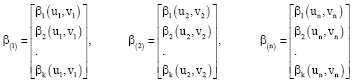
| (1) |
where, (uivi) denotes the co-ordinates of i-th point in space and βk(uivi) is the local coefficient for the k-th explanatory variable at location i.
The location-specific regression coefficients βk(uivi) are functions of longitude and latitude coordinates ui and vi. More precisely βk(uivi) is a realisation of continuous function βk(uivi) at point i. The local parameters βk(uivi) are estimated by weighted least-squares procedure. The weights wij are defined by a function of distance dij between a specific point j in the space at which data are observed and any point i in the space from which parameters are estimated.
The GWR approach gives more weights to data from observations close to i: data near to point i have more influence in the estimation of the βk(uivi)’s than do the data located farther from i. Similar to kernel regression and kernel density estimation, the GWR estimates location-specific parameters using weighted least square estimation; the only exception regards the weights: they are based on locations in geographic rather than attribute space. A number, say n, of unknown vectors of local regression coefficients are to be estimated:
 |
The GWR estimates of the unknown local parameter vector β(i) are given by:
| (2) |
which provides estimates for each variable k and each geographical location i. In Eq. 2, W(i) is the nxn spatial weight matrix which has the form:
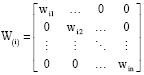 |
and whose diagonal elements are the weights of each observation. For example, wi1 is the weight of point 1 on the calibration of the model around point i. Thus the weighting of an observation is not longer constant in the calibration but varies with different locations. In the GWR framework, several weighting functions (kernels) can be considered and calibrated (Fotheringham et al., 1998) for calculating the weighted least-squares estimators (2), although they tend to be Gaussian or Gaussian-like, reflecting the type of dependency found in most spatial processes. Whichever weighting function is used, the results will be sensitive to the degree of distance-decay (bandwidth). As the bandwidth increases, the parameter estimates tend to the estimates from a global model. In some parts of the region, where data are sparse, the local regressions may be based on relatively few data points and may not estimate the parameters reliably. Conversely, fixed kernels in regions where data are dense may suffer from bias when the kernel are larger than needed. In order to avoid this problem, spatially adaptive weighting functions can be incorporated: these functions would have relatively small bandwidths in regions with high density of data points and larger in regions with low density of data points. Optimal bandwidth selection is a trade-off between bias and variance: too small a bandwidth leads to large variance in the local estimates; too large a bandwidth leads to large bias in the local estimates. Currently, Cross-Validation (CV) procedure, Generalised Cross-Validation (GCV) criterion of Loader (1999) or AIC (Akaike Information Criterion) (Hurvich et al., 1998) are generally employed to select the finest value of bandwidth.
CALIBRATING A LOCAL SPATIAL INTERACTION MODEL BY MEANS OF THE GWR
From previous section, it is possible to argue that GWR provides a framework for evaluating how the strengths of relationships change with the spatial resolution of the analysis. Examples of application of GWR can be found in a variety of disciplines (health, social science, economy, urban economics), where it has been also applied as a graphical tool for data exploration. By contrast, there are few attempts to measure local variations in spatial interaction modelling (Nakaya, 2001). This neglect may be because spatial interaction models are more complex than models for the geographic distribution of attribute data, with each region being associated with several values as an origin as well as a destination. It is worth stressing that the spatial disaggregation of spatial flows constitutes one of the earliest examples of providing local information on relationships (Fotheringham and O’Kelly, 1989). In this study, we propose a local calibration procedure for handling varying parameter estimates of an origin-constrained spatial interaction model. Suppose we deal with a spatial system consisting of m origin regions and n destination regions. Let, yij denote observations on independent random variables, say yij, (where, i denotes the origin regions and j the destination regions) sampled from a specified probability distribution dependent upon some mean (today’s prevailing specification is Poisson regression). The statistical spatial interaction model takes the general form as follows:
| (3) |
where the mean μij could be specified as a function of covariates measuring the characteristics of origin regions, destination regions and their separation (Bailey and Gatrell, 1995). The origin-constrained model, which reflects destination effect and distance frictional effect, takes the general form as follows:
| (4) |
where, v(xj; θ) is usually a linear function of the vector of destination characteristics (destination attractiveness); θ is a vector of associated parameters; the notation dij is used to represent the distance between i and j; γ is a distance deterrence effect; α is the balancing factor to ensure the origin constraint on predicted flows. It is worth noting that in the spatial interaction context the estimates of local parameters depend both on origins and destinations. Hence, the understanding of spatial interaction local interactions can be difficult as a four dimensional space is involved: the geographical space in which flow origins and flow destinations are located. One way to derive a suite of local parameters could be to use the conventional approach of spatial interaction model separately for each origin in the spatial system of interest. This leads to recast the origin-constrained model outlined above as:
| (5) |
Local parameters can be obtained by the maximisation of a weighted maximum likelihood function, exploiting the same principle of Geographical Weighted Regression (GWR) approach, using an iterative algorithm, implemented with an ad hoc R routine. In Eq. 5 the parameters have the index of origin i, as they are calibrated using flows from each origin separately; the index between brackets indicates that the application of GWR principle refers only, for simplicity, to the destination locations. For each destination location, the log-likelihood for the model in Eq. 5 includes the geographical weights and it is specified as follows:
| (6) |
As previously pointed out, the crucial issue regards the specification of the weighting function. The role of the weighting matrix in GWR is to represent the importance of individual observations among locations. Generally, the weight is determined by spatial distance only: it should decrease as difference between the focal point and its neighbours increases. One of the most commonly used spatial weighting function is the exponential distance-decay function:
| (7) |
Function in Eq. 7 produces a decay of influence with distance. If j and k coincide, the weighting of data at that point will be the unity. The weighting of other data will decrease according to a Gaussian curve, as distance between j and k increases. This function has received many other specifications (Brunsdon et al., 1996):
In this study we propose a modified version of weighting function which takes into account both the spatial distance and a function of strength of connection between two specific destinations. We assume that destinations which share more visitors tend to be more connected. Accordingly, we suggest the following format for the weighting function:
| (8) |
The strength of connection between two specific destinations is defined by:
where, ykj is the flow between k and destination j; yok and yoj denote the total flows of k and destination j respectively. We expect that the introduction in the weighting function of the strength of connection function can improve the model’s ability to replicate the known matrix flow. In order to evaluate the effects of our approach on the estimates, the local spatial interaction models with spatial and spatial-strength of connection weighting functions are compared.
A review of spatial interaction literature suggest that it is possible to draw proper conclusion regarding model performance examining the values of goodness-of-fit measures. In this study, we make use of a combination of two statistics: the Standardised Root Mean Square Error (SRME) and the Information Gain (Knudnes and Fotheringham, 1986; Fotheringham and Knudnes, 1987). The first statistics is calculated as follows:
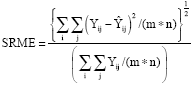 | (9) |
where, Yij is the observed number of people moving from region i to region j; ![]() are the estimated interactions between i and j and m and n are the number of origin and destination zones, respectively. The SRME statistic has a lower limit of zero, indicating perfectly accurate predictions and an upper limit variable, depending on the distributions of Yij's, although, in practice, it is often 1. Instead, the information gain statistics is defined as:
are the estimated interactions between i and j and m and n are the number of origin and destination zones, respectively. The SRME statistic has a lower limit of zero, indicating perfectly accurate predictions and an upper limit variable, depending on the distributions of Yij's, although, in practice, it is often 1. Instead, the information gain statistics is defined as:
| (10) |
where,
and
This goodness-of-fit statistic measures the difference between two probability distributions. It has minimum at zero, indicating a completely accurate set of predictions; the value of IG increases with differences between the observed and predicted flows distributions. In detecting local spatial variations of migration flows here, it is assumed that the spatial weighting functions, under study, are applied equally at each calibration point. The bandwidth, equal to 100, is determined on the basis of previous studies of phenomenon.
EXPLORING SPATIAL VARIATIONS IN MIGRATION FLOWS PATTERNS
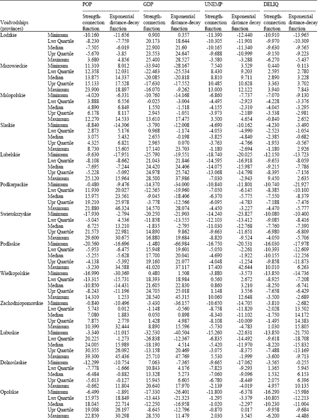
Here, we employ a spatial interaction approach to relate flows of migrants among Polish provinces to some potentially important explanatory variables. Polish internal migration flows for the single year of 2004 and the geographic resolution of NUTS-2 (the 16 Polish provinces or voidvodships) constitute the empirical basis of our analysis. The data used in this study are drawn from the Polish Official Statistic (Polka Statystyca Publiczna). The aim of this application is twofold. Firstly, we estimate parameters of a global origin-constrained spatial interaction model in order to select variables which determine the relative attraction of destinations. Economic variables (such as GDP per capita), labour market variables (such as levels of employment), environmental variables, embracing physical, economic, social and political aspects, are seen as potentially important. Along with the so-called gravity variables, population and physical distance, also the unemployment rate and per capita GDP are incorporated in the fitted models as covariates. Moreover a social explanatory variable, the rate of detectability of delinquents, is also added to the model to assess if better living conditions, in terms of social security, might have an impact on the migration process. Global research findings establish a substantial influence of economic factors on migration flows. The estimated coefficients for the unemployment rate and GDP per capita emphasise this aspect (Table 1, in which parameter coefficients are expressed in logarithms).
Secondly, a further purpose of this application concerns the formulation of two localised origin specific constrained models, to capture regionally different sensitivities of explanatory variables, exploiting the same principle of GWR. They rely on a different specification of weighting functions. In one of them, the weights are defined according to a common used Gaussian distance decay based function (Eq. 7); in the other, our proposed weighting function combining the geographical space and the strength of connection (Eq. 8) is adopted. The best way for understanding the geographical variations of parameters may be to build maps of local parameters. However, owing to the volume of output of local estimates, it is not possible to display all maps for each combination of origins and destinations. An informal but convenient indication of the extent of spatial non-stationarity in the local parameter estimates, has been obtained by assessing if the range of local estimates between the inter-quartile range is greater than that of 2 standard errors of the global estimates, as suggested in Fotheringham et al. (2002).
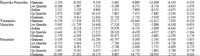
The main empirical findings, achieved by the calibration of the two localised origin-specific-constrained models, are summarised in Table 2, in which we set out for each sending region the median, the upper and lower quartiles and the minimum and maximum values of the estimated parameters, got from the estimates over all destination provinces. In Table 2, we do not display the distance decay exponent, whose impact is stable across the study region. The analysis of the overall results shows local anomalies of parameters drifts in some region, particularly in the area of capital Warszawa (Mazowieckie voidvodship). Particular attention is paid to the main economic determinants of migration flows: the unemployment rate and per capita GDP. Regarding that, it is interesting to point out that while the global coefficient signs confirm that migrants are willing to move towards provinces characterised by low unemployment rate and high per capita GDP, the local estimates shows some counter-intuitive results.
| Table 1: | Global origin-constrained model coefficients |
 | |
| Table 2: | Summary statistics of estimated parameters for localised origin-specific–constrained models with different weighting functions |
 | |
 | |
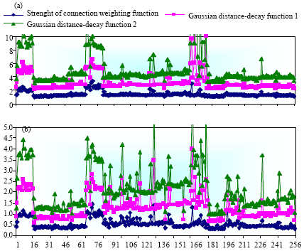 | |
| Fig. 1: | Measures of predictive performance of localised specific origin-constrained models with different weighting functions |
It should be noted that the geographical parameter drifts are strongly dependent on the combinations of origins and destinations. This makes very difficult to deeply recognize the determinants of people movements. Finally, to further illustrate the effect of our specification of the weighting function on the models ability in replicating the observed flow data, we calculate and compare two different goodness-of-fit statistics (SMRE and IG), as defined here. The potential advantages arising from the introduction of the function of strength of connection in the weighting scheme, are evaluated by the comparison with the following different Gaussian weighting functions:
and
indicated in Fig. 1 as Gaussian distance decay function 1 and Gaussian distance decay function 2, respectively.
The parameters of coefficients, estimated in each of the destination provinces and for each of the sending provinces allow us to obtain 256 matrices of predicted flows to be compared with the observed flows among Polish voivodeships. The results, obtained from the local spatial interaction models under study, indicate a better prediction power for the model with the new weighting function, through which we constantly observe smaller values of both the considered Standardised Root Mean Square Error and Information Gain statistics (Fig. 1). It implies that local spatial interaction model fits the data better if the spatial-strength of connection weighting function is used.
CONCLUSIONS
Although, applications of GWR can be found in a variety of disciplines, there are few efforts to document local variation of spatial interaction models. In this study, exploiting the same principle of GWR, we obtained the parameters drifts for localised origin-specific-constrained models. In the GWR approach, there are many options regarding the specification of the weighting function. Currently, the geographical weight designates the degree of spatial separation between the focal point and its neighbours. In this study, we recommend a diverse weighting function which includes both the geographical distance and the strength of connection between two regions, properly specified. Migration flows among Polish provinces are used as an illustrative application of the suggested approach. The obtained localised parameters exhibit a high degree of variability over space and demonstrate complex spatial patterns of the variables. We expected that the introduction in the weighting scheme of Athe strength of connection@ between two specific localisations could improve the prediction power of the model. In this regard, we compared the overall performance of our localised spatial interaction model, in terms of prediction errors, with localised spatial interaction models where the weighting functions are taken in the traditional Gaussian distance-decay form. The lower values of both goodness-of-fit statistics employed represent empirical evidence that the introduction of new weighting function has significantly improved the model’s ability in replicating the known matrix flows. In some way, the improvements of fitting can be regarded as an alternative way to detect the presence of spatial relationship, validating the usefulness of our proposed approach for handling varying parameters estimates of spatial interaction models.
REFERENCES
- Anselin, L., 1995. Local indicators of spatial association-LISA. Geograph. Anal., 27: 93-115.
CrossRefDirect Link - Brunsdon, C.F., A.S. Fotheringham and M.E. Charlton, 1996. Geographically weighted regression: A method for exploring spatial nonstationarity. Geographical Anal., 28: 281-298.
CrossRefDirect Link - Casetti, E., 1972. Generating models by expansion method: Applications to geographical research. Geographical Anal., 4: 81-91.
CrossRefDirect Link - Chun, Y., 2008. Modeling network autocorrelation within migration flows by eigenvector spatial filtering. J. Geographical Syst., 10: 317-344.
CrossRefDirect Link - Fischer, M.M. and D.A. Griffith, 2008. Modelling spatial autocorrelation in spatial interaction data: An application to patent citation data in the European union. J. Regional Sci., 48: 969-998.
CrossRefDirect Link - Fotheringham, A.S., 1983. A new set of spatial interaction models: The theory of competing destinations. Environ. Plann. A, 15: 15-36.
Direct Link - Knudnes, C.D. and A.S. Fotheringham, 1986. Matrix comparison, goodness-of-fit and spatial interaction modeling. Int. Regional Sci. Rev., 10: 127-147.
CrossRefDirect Link - Fotheringham, A.S., M.E. Charlton and C.F. Brunsdon, 1998. Geographically weighted regression: A natural evolution of the expansion method for spatial data analysis. Environ. Plann. A, 30: 1905-1927.
Direct Link - Hurvich, C.M., J.S. Simonoff and C.L. Tsai, 1998. Smoothing parameter selection in nonparametric regression using an improved Akaike information criterion. J. R. Stat. Soc. Ser. B, 60: 271-293.
Direct Link - Le Sage, J., M.M. Fischer and T. Scherngell, 2007. Knowledge spillovers across Europe: Evidence from a Poisson spatial interaction model with spatial effects. Papers Regional Sci., 86: 393-421.
CrossRef - Nakaya, T., 2001. Local spatial interaction modelling approach based on the geographically weighted regression approach. GeoJ., 53: 347-358.
CrossRefDirect Link - Jim, P., 1998. Competition among destinations in spatial interaction models: A new point of view. Chinese Geographical Sci., 8: 212-224.
CrossRefDirect Link - Tiefelsdorf, M., 2003. Misspecifications in interaction model distance decay relations: A spatial structure effect. J. Geographical Syst., 5: 25-50.
CrossRefDirect Link