Optimal Computerized Model for Designing Cellular Manufacturing Systems using Neural Network

INTRODUCTION

Group Technology (GT) is a manufacturing management philosophy that emphasizes on identifying groups of products with similar design and processing characteristics. Cellular Manufacturing (CM) is an application of GT that attempts to identify a collection of similar parts (part families) which can be processed in a manufacturing cell with dissimilar machines. Such an arrangement of machines facilitates complete processing of part families within the manufacturing cell (Panchalavarapu and Chankong, 2005).

Akturk and Balkose (1996) stated that group technology is one of the most important aspects in the design of Cellular Manufacturing Systems (CMS). It has been realized that GT based CMS have benefited from the advantages of both product-based manufacturing systems and job shop manufacturing systems (Soleymanpour et al., 2002). CM is an effective means of efficiently producing small batches of a large variety of part types. A key step in CM is manufacturing cell formation, i.e., grouping parts with similar design features or processing requirements into families and allocating associated machines, forming cells. The similarity among the parts in each family allows for significant set-up reductions, leading to smaller economic lot sizes and lower work-in-process inventories (Dobado et al., 2002). Generally, the cell formation problem can be represented in matrix format by using a ‘machine-part incidence matrix’ in which all the elements are either zero or one. A one element indicates that a specific machine is used to process a specific part and zero element indicates the opposite (Sarker and Islam, 2000). The problem is equivalent to block diagonal sing a zero-one input matrix. Grouping of components into families and machines into cells result in a transformed matrix with diagonal blocks where ones occupy the diagonal blocks and zeros occupy the off-diagonal blocks. The resulting diagonal blocks represent the manufacturing cells (Nair and Narendran, 1998). The case where all the ones occupy the diagonal blocks and all the zeros occupy the off-diagonal blocks is called perfect diagonal blocks. But this case is rarely accomplished in practice. For that, the most desirable solution of cellular manufacturing systems is that which gives minimum number of zero entries inside a diagonal block (known as voids) and minimum number of one entries outside the diagonal blocks (known as the exceptional elements). A void indicates that a machine assigned to a cell is not required for the processing of a part in the cell. An exceptional element is created when a part requires processing on a machine that is not available in the allocated cell of the part. Voids and exceptional elements have adverse implications in terms of system operations (Adil et al., 1996).

The main objective in CM is to identify machine cells and part families such that every part undergoes almost all of its processing in the assigned machine cell. Cell Formation (CF) is considered to be the first step in CM design. CF is recognized by researchers as a complex problem. The size of the engineering problem of CM philosophy can be looked at from many important characteristics such as: Number of cells, cell size, operation sequence, process plan and machine loading/balancing (Srivastava and Chen, 1995). Lee et al. (2010) suggested a heuristic approach to the machine loading problem in order to reduce the maximum workload of the machines by partially grouping them.

Many researchers mentioned that little research has been done to determine the optimal number of cells and that it is usually left as a managerial or facility designer decision. Several authors have developed and published solution methods to generate cell formation. Specifying the number of cells in advance and obtaining all the natural clustering of the input matrix, can be achieved by developing algorithms or models that take all the possible ways of forming p-cells from n-machines. Niknam et al. (2008) used a hybrid evolutionary optimization algorithm based on Ant Colony Optimization (ACO) and Simulated Annealing (SA) for optimal clustering N object into K clusters.

Since the problem of the cell formation is considered to be complex, many researchers worked on to develop a solution using Artificial Neural Network (ANN). The ANN is an efficient method that can be used in CF regardless the number of machines and parts. Using ANN in cell formation will make the processing time needed only few seconds. Sivaprakasam and Selladurai (2008) used Memetic Algorithm (MA) with Gentic Algoritm (GA) to minimize the exceptional elements.

Artificial Neural Networks (ANN’s) have received a lot of attention in recent years due to their attractive capabilities in forecasting, modeling of complex nonlinear systems and control. Applications of neural networks include many various fields among which are engineering and business. ANN’s have been used for forecasting electric load (Kalaitzakis et al., 2002), gasoline consumption (Nasr et al., 2003), energy (Reddy and Ranjan, 2003) and financial indicators (Chen et al., 2003; Tkacz, 2001).

Artificial neural networks are widely used for forecasting. A large number of successful applications have shown that neural networks can be a very useful tool for time series modeling and forecasting (Zhang et al., 1998). In addition, the simulation experiments of Zhang et al. (2001) show that neural networks are valuable tools for forecasting nonlinear time series when compared to other traditional linear methods. Even though it may sound that ANN’s are not needed for modeling and forecasting linear time series due to the well developed linear system theory, they are competent in Zhang (2001). The ANN model is trained with historical time series input-output process data or observations and is then used to predict the output in the future.

In this study, a special model for generating a three-cell formation is developed with minimum sum of voids (v) and/or exceptions (e). The computerized model is designed for the case of unbounded cell size that takes all the possible ways of forming 3-cells from n-machines by using Artificial Neural Networks (ANN). The output of the computerized model will be input to the ANN. For small number of machines the computerized model can generate all the possible ways of forming three cells from n machines and then find the optimal number of exception (e) plus voids (v) (e+v). For large number of machines the computerized model can generate only all the possible ways of forming three cells from n machines, since it is impossible to run the program to find the optimal (e+v). In this case the output of the generation of large number of machines will be input to the ANN.

The main objective of this study is to determine the exact and optimal solution (s) of forming three cells from any number of machines by using ANN. The significance of this model is that, the processing time needed to run the program (the output of the computerized model) takes only few seconds because machine cells and part families are identified and done concurrently which will decrease the computational time. Machine cells and part families are identified so as to minimize the sum of voids (v) and/or exceptions (e) according to the designer wish. Moreover, the designer will get more flexibility in choosing between different cells.

Table 1:	Computerized model to compute the optimal value of exceptions (e) plus voids (v) (e+v)

Table 2:	Computation of the e+v value

COMPUTERIZED MODEL

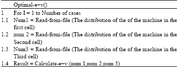
The method describes distributing the machines in three different cells in all possible way. Table 1 contains the computerized model that computes the optimal value of exceptions (e) plus voids (v) (e+v). It takes the distributions of the machines in three different cells and computes the optimal value for each case at the end we store this value in the Result parameter. The complexity of this algorithm is O (m*n) where m is the number of cases and n is the number of machines.

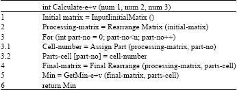
Calculate-e+v () algorithm presented in Table 2. The function Input Initial Matrix () in line 1 presents any matrix input by the user (according to designer) that distribute machines in three different cells. Rearranging the initial matrix according to the three input numbers by using the Rearrange Matrix () function in line 2 and the result stores in the processing- matrix.

Passing the processing- matrix and the part-no to the function Assign Part () presented in line 3 (3.1, 3.2) that responsible to assign each part in its corresponding cell based on the minimum e+v among the different cells. The function Final Rearrange () rearranges the matrix in the final form according to parts distribution among cells (line 4). Then the Get Min-e+v() (line 5) computes the minimum value of e+v for the specific distribution.

NEURAL NET MODELING

Artificial neural networks were originally inspired as being models of human nervous system. They have been shown to exhibit many abilities, such as learning, generalization and abstraction (Patterson 1990). Useful information and theory about ANN’s can be found by Haykin (1999). These networks are used as models for processes that have input-output data available. The input-output data allows the neural network to be trained such that the error between the real output and the estimated (neural net) output is minimized. The model is then used for different purposes among which are estimation and control.

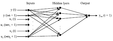
The Artificial Neural Net (ANN) structure is shown in Fig. 1 with a multi-input single-output. The inputs feed forward through a hidden layer to the output. The hidden layer contains processing units called nodes or neurons. Each neuron is described by a nonlinear sigmoid function. The inputs are linked to the hidden layer which is in turn linked to the output. Each interconnection is associated with a multiplicative parameter called weight. Note that the feed-forward neural net of Fig. 1 has only one hidden layer and this is the case that we are going to consider. A number of results have been published showing that a feed-forward network with only a single hidden layer can well approximate a continuous function (Cybenko, 1989; Funahashi, 1989). In practice, most of the physical processes are continuous.

An artificial neural net mathematical model that represents the structure shown in Fig. 1 is written as:

(1)

where, y_nn (t + 1) is the output of the neural net model, U is a column vector of size N that contains the inputs to the ANN, W_o is a row vector of size h that contains the output weights from the hidden layer to the output with h being the number of hidden nodes, W_i is a matrix of size hxN that contains the input weights from the inputs to the hidden layer, B_i is a column vector of size h that contains the input biases and b_o is the output bias. Note that tanh (W_i *U + B_i) is the activation function of the hidden layer. It is a column vector of size h.

The weights and biases of the ANN are determined by training with the historical input-output data. Backpropagation is an example of a training algorithm. For a given number of hidden neurons the network is trained to calculate the optimum values of the weights and biases that minimize the error between the real and ANN outputs. We assume that after an appropriate choice of the number of hidden neurons and a suitable training period, the network gives a good representation of the estimation system given in Eq. 1.

Fig. 1:	Neural net structure

SIMULATION RESULTS

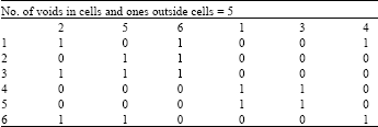
To illustrate and test the proposed model, the researchers will apply it on an industrial problem cited by Chen and Cheng (1995). Who solved by using Adaptive Resonance Theory (ART1). Table 3 shows the machine-part matrix to the problem consisting of 6•6 machine-part. To validate and verify the proposed model, this problem will be solved and the result will be compared with their solution.

Since we have 6 machines, then all the possible ways to distribute 6 machines to form 3 cells is equal to 90 ways (Mukattash, 2000).

Based on the model developed input-output data will be generated. The data contains 90 patterns. Each pattern includes data about the 3 inputs: the machines in each of the 3 cells and corresponding output e+v.

The 90 data patterns are used to train an artificial neural net model for the process. The training was done with the software package Matlab. Experiments were run for different numbers of hidden neurons.

It was observed that the quality of the results depends on the number of hidden neurons. The square error, S, is defined as:

(2)

where, M is the number of data points which is equal to 90 in our case, y_nn is the neural net output and y_r is the real output. Recall that the output is the e+v value.

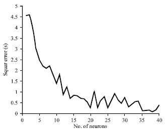
The square error (S) is plotted as a function of the number of hidden neurons in Fig. 2. Note that this function is decreasing. The square error almost settles at a small value when the number of neurons is large enough. By inspecting Fig. 2, the neural net with 20 hidden neurons was selected as the optimum net. The corresponding square error is equal to 0.1111. For nets much larger than 20 hidden neurons the square error decreases further but makes the neural net large involving large number of parameters which causes the undesirable over-fitting of data.

Fig. 2:	The least square error as a function of the number of hidden neurons in the neural net

Table 3:	Part list and machines

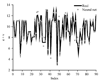
The real output (voids + exceptions, e+v) and the optimum (20 hidden neurons) neural net approximated output are plotted in Fig. 3. Note that the two outputs are very close to each other. This indicates the accuracy of the selected neural net. Therefore, the neural net can be relied on to locate the optimum e+v value which is of great practical importance. The complete solution of this problem is shown in Table 5. Machine cells and part families are identified in this problem so as to minimize the sum of voids and exceptions.

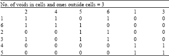
Table 4 shows the solution of the problem in Table 3 using Adaptive Resonance Theory (ART1). It is clear that there is two voids and two exceptions (e+v = 4) and this solution supposed to be optimal. Table 5 shows the solution used the proposed model. Comparing Table 4 with 5, it can be concluded that the proposed model gives better result than ART1model since there are three exceptions and no voids. (e+v = 3).

Table 4:	ART1 solution

Table 5:	Proposed model solution

Fig. 3:	The selected optimum neural net training results

Also this result (e+v = 3) is optimal since any other cell formation will not give (e + v) less than 3.

REFERENCES

- Akturk, M.S. and H.O. Balkose, 1996. Part-machine grouping using a multi-objective cluster analysis. Int. J. Product. Res., 34: 2299-2315.
CrossRefDirect Link - Chen, A.S., M.T. Leung and H. Daouk, 2003. Application of neural networks to an emerging financial market: Forecasting and trading the Taiwan Stock Index. Comput. Operat. Res., 30: 901-923.
CrossRefDirect Link - Chen, S.J. and C.S. Cheng, 1995. A neural network-based cell formation algorithm in cellular manufacturing. Int. J. Product. Res., 33: 293-318.
CrossRef - Dobado, D., S. Lozano, J.M. Bueno and J. Larraneta, 2002. Cell formation using a fuzzy min-max neural network. Int. J. Product. Res., 40: 93-107.
CrossRefDirect Link - Funahashi, K.I., 1989. On the approximate realization of continuous mappings by neural networks. Neural Networks, 2: 183-192.
CrossRefDirect Link - Lee, J., C.O. Malave, T.S. Kim and S.J. Lee, 2010. A heuristic approach for workload balancing problems. Asian J. Ind. Eng., 2: 1-8.
CrossRefDirect Link - Kalaitzakis, K., G.S. Stavrakakis and E.M. Anagnostakis, 2002. Short-term load forecasting based on artificial neural networks parallel implementation. Electric Power Syst. Res., 63: 185-196.
CrossRef - Mukattash, A., 2000. Generation of three-cell formation algorithm with minimum sum of voids and exception. Dirasat, Eng. Sci. Univ. Jordan, 27: 96-109.
Direct Link - Nair, G.J. and T.T. Narendran, 1998. Case a clustering algorithm for cell formation with sequence data. Int. J. Prod. Res., 36: 157-180.
Direct Link - Niknam, T., J. Olamaei and B. Amiri, 2008. A hybrid evolutionary algorithm based on ACO and SA for cluster analysis. J. Applied Sci., 8: 2695-2702.
CrossRefDirect Link - Panchalavarapu, P.R. and V. Chankong, 2005. Design of cellular manufacturing systems with assembly considerations. Comput. Indust. Eng., 48: 449-469.
CrossRef - Reddy, K.S. and M. Ranjan, 2003. Solar resource estimation using artificial neural networks and comparison with other correlation models. Energy Conversion Manage., 44: 2519-2530.
Direct Link - Sarker, B.R. and K.M.S. Islam, 2000. A similarity coefficient measure and machine parts grouping in cellular manufacturing systems. Int. J. Prod. Res., 38: 699-720.
Direct Link - Sivaprakasam, R. and V. Selladurai, 2008. A memetic algorithm approach for minimizing exceptional elements in cell formation. Asian J. Scientific Res., 1: 138-145.
CrossRefDirect Link - Srivastava, B. and W. Chen, 1995. Efficient solution for machine cell formation in group technology. Int. J. CIM., 8: 255-264.
CrossRefDirect Link - Soleymanpour, M., P. Vrat and R. Shankar, 2002. A transiently chaotic neural network approach to the design of cellular manufacturing. Intl. J. Prod. Res., 40: 2225-2244.
Direct Link - Tkacz, G., 2001. Neural network forecasting of Canadian GDP growth. Int. J. Forecast., 17: 57-69.
CrossRef - Zhang, G., B.E. Patuwo and M.Y. Hu, 1998. Forecasting with artificial neural networks: The state of the art. Int. J. Forecast., 14: 35-62.
CrossRefDirect Link - Zhang, G.P., G.E. Patuwo and M.Y. Hu, 2001. A simulation study of artificial neural networks for nonlinear time-series forecasting. Comput. Operat. Res., 28: 381-396.
CrossRefDirect Link - Zhang, G.P., 2001. An investigation of neural networks for linear time-series forecasting. Comput. Operat. Res., 28: 1183-1202.
CrossRef - Cybenko, G., 1989. Approximation by superpositions of a sigmoidal function. Mathe Control Signals Syst., 2: 303-314.
CrossRefDirect Link - Nasr, G.E., E.A. Badr and C. Joun, 2003. Backpropagation neural networks for modeling gasoline consumption. Energy Convers. Manage., 44: 893-905.