
A.N. H. Alnuaimy
Department of Electrical, Electronic and Systems Engineering, Faculty of Engineering and Built Environment, National University of Malaysia, 43600 UKM Bangi Selangor Darul Ehsan, Malaysia
M. Ismail
Department of Electrical, Electronic and Systems Engineering, Faculty of Engineering and Built Environment, National University of Malaysia, 43600 UKM Bangi Selangor Darul Ehsan, Malaysia
M.A. M. Ali
Department of Electrical, Electronic and Systems Engineering, Faculty of Engineering and Built Environment, National University of Malaysia, 43600 UKM Bangi Selangor Darul Ehsan, Malaysia
K. Jumari
Department of Electrical, Electronic and Systems Engineering, Faculty of Engineering and Built Environment, National University of Malaysia, 43600 UKM Bangi Selangor Darul Ehsan, Malaysia
Journal of Applied Sciences
Year: 2009 | Volume: 9 | Issue: 18 | Page No.: 3371-3377


ABSTRACT
In an improved algorithm of channel estimations of Orthogonal Frequency Division Multiplexing (OFDM) system based pilot signal, the channel will be estimated using the mean and the variance of the two adjusted channel samples which have been extracted from that those embedded pilot signal in given positions of the frequency-time grid of OFDM signals. In this study, we present the application of Trellis Code Modulation (TCM) over an improved algorithm of the of the channel estimation of OFDM system based pilot signal and the usage of wavelet de-noising filter for that estimated channel sample to reduce the noise which affect the estimation of the channel. Simulation results shows that the combination of the TCM and the Wavelet de-noising filter will increase the performance of the OFDM system over that improved algorithm for the channel estimations.
PDF Abstract XML References Citation
How to cite this article
A.N. H. Alnuaimy, M. Ismail, M.A. M. Ali and K. Jumari, 2009. TCM and Wavelet De-Noising Over an Improved Algorithm for Channel Estimations of OFDM System Based Pilot Signal. Journal of Applied Sciences, 9: 3371-3377.
DOI: 10.3923/jas.2009.3371.3377
URL: https://scialert.net/abstract/?doi=jas.2009.3371.3377
DOI: 10.3923/jas.2009.3371.3377
URL: https://scialert.net/abstract/?doi=jas.2009.3371.3377
INTRODUCTION
The OFDM is a digital multi-carrier modulation scheme, which uses a large number of closely-spaced orthogonal sub-carriers that is particularly suitable for frequency-selective channels and high data rates. This technique transforms a frequency selective wide-band channel into a group of non-selective narrow-band channels, which makes its robust against large delay spreads by preserving orthogonality in the frequency domain as in frequency selective fading channels wideband signals suffer inter-symbol interference while those narrowband signals only experience at fading. Orthogonal Frequency Division Multiplexing (OFDM) systems are especially suited for channel estimation. In order to achieve the potential advantages of OFDM systems, the channel coefficients should be estimated carefully.
Channel estimation is an important and necessary function for modern wireless receivers which can be improved using more pilot symbols (Slock, 2004). With even a limited knowledge of the wireless channel properties, a receiver can gain insight into the information that was sent by the transmitter. The goal of channel estimation is to measure the effects of the channel on known or partially known transmissions, where the channel samples will be extracted from those known pilot signal and using a proper interpolation method for accurate estimation of the channel.
In general OFDM systems, pilots can be sent either in block or comb-type arrangements. In block-type arrangement, pilots are sent on every sub-carrier in a time-periodic manner. In comb-type, pilots are sent continuously in a frequency-periodic manner.
After the estimation of the channel transfer function of pilot tones, the channel transpose of data tones can be interpolated according to adjacent pilot tones. The linear interpolation has been studied in (Rinne and Renfors, 1996) and is shown to be better than piecewise constant interpolation. The other most general methods of interpolation used for the estimation of the channel over OFDM system is:
| • | Linear interpolation |
| • | Spline interpolation |
| • | Cubic interpolation |
In this study, wavelet de-noising filter will be used in order to reduce the effect of the noise over the estimated channel using an improved algorithm for the channel estimation of OFDM system (Ahmed et al., 2009) which use a as specific pilot signal arrangement different form comb and block type as can be seen later. As the joint of improved algorithm and wavelet de-noising can bring to more accurate estimation. Also, Viterbi detection will be used in order to reduce the effect of the noise over the original transmitted signal.
SYSTEM MODEL
The transmitter and receiver of the OFDM system over pilot insertion block, TCM and wavelet de-noising filter will be described.
Transmitter structure: As shown in Fig. 1, the vector of data s is encoded and mapped according to 2/3 convolutional coding over 8-PSK for TCM (Ungerboeck, 1987). Then, for pilot symbol aided channel estimation, Nf and Nt pilot symbols are inserted periodically with the distance Df and Dt in frequency and time grid respectively with the insertion of a single pilot sample of the last sample of each symbol adjacent to the uniformly distributed pilot samples symbol, as shown in Fig. 2, as the serial vector of the result data converted to N×K vectors by a serial-to-parallel converter where N is the number of total sub-carriers in one OFDM symbol and K is the total number of OFDM symbols in the frame.
 | |
| Fig. 1: | Transmitter structure of the OFDM system |
 | |
| Fig. 2: | Pilot distribution for OFDM system in frequency-time grid |
At this time, each OFDM symbols vector in the frame xN= [x1(k) x2 (k) x3(k)… xN(k)] will be modulated using N point Inverse Fast Fourier Transform (IFFT). At the terminal end of the transmitter, the resulted OFDM vector in the frame will be sent serially through the time varying frequency selective channel. The channel will be described using baseband equivalent impulse response as h(k) = [ h1(k) h2(k) … hLf (k)]T where Lf is the length of channel (Coleri et al., 2002). The channel is modeled as an impulse response h(t) followed by the complex Additive White Gaussian Noise (AWGN) n(t):
| (1) |
where, αm is a complex values and Ts is the sampling interval.
Receiver structure: At the receiver side as shown in Fig. 3, the received signal will be demodulated using N point (FFT), where the resulted signal will be as follow:
| (2) |
where, nn(k) is the FFT sample of the additive white Gaussian noise and Hn(k) is the frequency domain of the channel coefficient for the nth sub-carrier and the kth OFDM symbol.
The channel sample will be extracted from the received pilot signal by using LS channel estimation in frequency domain as the receiver know the sample at that signal as:
| (3) |
where, xp(k) is the pilot sample in the OFDM signal, is the coefficient of the channel at that pilot sample (Biglieri et al., 1998). Where the channel coefficient will be filtered using a wavelet de-noising as it can be seen in Fig. 3, then estimation of the channel will be done which is used to be combined with received signal to reduce the channel from that signal which will be passed through ML detection using Viterbi algorithm (Viterbi, 1967), to get the final signal.
 | |
| Fig. 3: | Receiver structure of OFDM system |
An improved algorithm for channel estimation based on pilot sample: Using those extracted channel coefficients at that pilot to estimate the channel coefficients for the OFDM signal. In order to obtain estimated channel coefficients for all sub-carriers the mean and the variance of two adjacent channel coefficient extracted from those pilot samples and then using the equation of the mean and variance to calculate the estimated channel coefficients as follow:
| • | Calculating of the mean and the variance of the two channel coefficient which has been extracted from the pilot sample in the same time period of OFDM symbol as follow: |
| (4) |
| (5) |
where, Np is the number of pilot used in the equation.
| • | Multiplying the calculated variance by a factor ξ where ξ=0.556 |
| • | Calculating the value of the two entire samples between the two pilots using the following equation: |
| (6) |
where, he is the estimated coefficient of the channel, while c1 and c2 will be calculated as follow:
| (7) |
| (8) |
| • | Now for the calculation of the channel coefficient between OFDM symbol the same cited procedure will be used but with aid of the past calculated coefficient to calculate the mean and the variance and modified by α and β factor respectively. Where α and β factor will be explained with aid of schemes. In this study we will propose that those factors will be known |
α and β factors: α and β factors are the modification factor for the mean and variance of the two adjacent pilot sample of the same sub-carrier of the OFDM symbols. Where these two factors are limited to unity value as those factor are fluctuated around the value of one. By testing the Probability Density Function (PDF) of these factors it was found that these two factors limited to one as the doppler frequency fd dencrease as shown in Fig. 4, 5 which can show the normal distribution of 4, 6 and 8 tab of the channel length for both of α and β factors (mean and variance factor, respectively).
Wavelet de-noising: Wavelet analysis is capable of revealing aspects of data that other signal analysis technique as fourier analysis which miss aspects like trends, breakdown points, discontinuities in higher derivatives and self-similarity.
 | |
| Fig. 4: | Probability density function of α factor for different doppler frequency of the channel |
 | |
| Fig. 5: | Probability density function of β factor for different doppler frequency of the channel |
Furthermore, because it affords a different view of data than those presented by traditional techniques, wavelet analysis can often compress or de-noise a signal without appreciable degradation.
Fourier analysis has a serious drawback. In transforming to the frequency domain, time information is lost. When looking at a fourier transform of a signal, it is impossible to tell when a particular event took place.
Wavelet de-noising can bring to more accurate estimation for the channel by reducing the effect of the noise on the estimated channel. As the noisy channel coefficients pass through the wavelet de-noising filter the estimated signal will be more accurate as shown in Fig. 6. The general wavelet de-nosing procedure is as follows (Wang et al., 2000):
| • | Apply wavelet transform to the noisy signal to produce the noisy wavelet coefficients to the level which we can properly distinguish the PD occurrence |
| • | Select appropriate threshold limit at each level and threshold method (hard or soft threshold) to best remove the noises |
| • | Inverse wavelets transform of the thresholded wavelet coefficients to obtain a de-noised signal |
The threshold is crucial when use the wavelet de-noising. Function wden in Matlab is used to remove (I +W)Xp*. The option minimaxi is used as threshold algorithm. It is presented in:
| (9) |
where, n is the length of the signal. It can be seen that the thr is directly proportional to the σ (D1) . So, the noisy is removed efficiently unless the threshold thr is chosen close to σ ((I +W)Xp*), the standard deviation of the noisy (I +W)Xp*. It means to minimize the Δ:
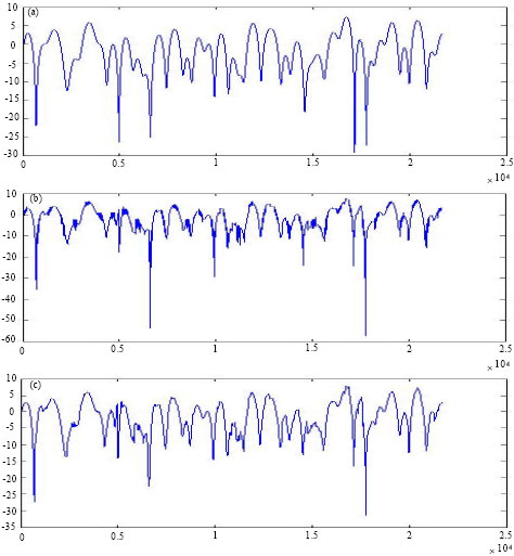 | |
| Fig. 6: | Estimated Channel over Wavelet De-noising filter, (a) Original fading channel , (b) Noisy estimated channel and (c) Estimated channel over Wavelet de-noising |
| (10) |
D1 is the first-level detail coefficients. We choose thr to make Δmin and use wavelet de-noising method to remove (I +W)Xp* to get more accurate.
Viterbi decoder: Soft Maximum-Likelihood (ML) decoding using the Viterbi-Algorithm (VA) is assumed (Viterbi, 1967). The Viterbi decoder divides the input data stream into blocks, estimating the most likely data sequence and outputting each decoded data sequence in a burst. The Viterbi algorithm performs the trace back operation in parallel with the path calculations. The width of the metric registers must be enlarged when using high rate punctured codes, when the number of bits used in soft decision is large and when the Bit Error Rate at the input of the Viterbi decoder is high. The trace back depth should be sufficiently long to avoid loss of accuracy, therefore 20 trace back depth was used in the simulation in order to get a good accuracy.
SIMULATION
Simulation parameter: In this study, the simulation has been considering different values of the doppler frequency for the Rayleigh fading channel according to the velocity of the vehicle with Additive White Gaussian Noise (AWGN). The channel is assumed to be frequency selective fading, where the doppler frequency for the channel has been calculated using:
| (11) |
where, fd is the doppler frequency, v is the vehicle velocity and c is the light speed. Table 1, shows the parameter specifications for OFDM system based on the trellis code modulation (TCM) and the wavelet de-noising filter.
Simulation results: Now, we will test different OFDM systems over different parameters of Rayleigh fading channel.
| Table 1: | Parameter of OFDM system base TCM and Wavelet de-noising filter |
 | |
Where the tested OFDM systems based on improved algorithm of channel estimation (C.C.), are OFDM system based on TCM (CCV), OFDM system based on wavelet de-noising (CCWden) and OFDM system based on both TCM and wavelet de-noising (CCVWden).
Figure 7 shows testing of the four OFDM systems over fixed parameter of the channel, 100 Hz doppler frequency has been selected for the Rayleigh fading channel in additional to AWGN for testing those different systems. As can be seen that OFDM/CCV can improve the performance of the system in both cases (with and without wavelet de-noising filter) by about 7.5-8 dB for all BER.
 | |
| Fig. 7: | Performance of different OFDM systems over 100 Hz doppler frequency of Rayleigh fading channel |
 | |
| Fig. 8: | Performance of different OFDM systems over different value of doppler frequency of Rayleigh fading channel |
 | |
| Fig. 9: | OFDM system based an improved algorithm for channel estimation, TCM and wavelet de-noising over different doppler frequency of the rayleigh fading channel |
While, the usage of the wavelet de-noising filter in both cases (with and without TCM) can improve the performance limitedly, while at 40 dB of SNR, BER will improved as for C.C. BER equal to 3×10⁻², while for C.C.Wden is about 3×10⁻³ so as for OFDM/C.C.V., where BER for the OFDM/C.C.V system without Wden at 40 dB of SNR, BER will be about 8×10⁻², while with Wden will be 8×10⁻².
Figure 8 shows testing of the four OFDM systems over different values of doppler frequency in addition to AWGN for testing those different systems. Where it is clear that the for the whole OFDM systems the BER of the each system increased by increasing of doppler frequency of the channel as the performance of the OFDM/CCV in both cases (with and without Wden) improve the performance of the system, while for that base Wden (with and without TCM) will increase the performance especially at high doppler frequencies of the channel.
Finally, Fig. 9 shows OFDM system based on an improved algorithm for channel estimation, TCM and wavelet de-noising over different values of doppler frequency. Where, it is obviously that the performance of that system increasing by the decreasing of the doppler frequency of the channel.
RESULTS AND DISCUSSION
From the simulation result, it was found that the OFDM/CCVWden give the pest performance of the OFDM system over the others as it can improve the performance by about 7-8 dB over OFDM/C.C., 6-7.5 dB over OFDM/CCWden as the performance of the system improved up to 10 dB by using the TCM and Viterbi decoder for error correction (Akay and Ayanoglu, 2004) and about 1.5-2 dB over OFDM/CCV.
 | |
| Fig. 10: | Coded and uncoded OFDM system over AWGN |
So, from Fig. 9, it is obvious that the OFDM/C.C.V.Wden performance increase as the doppler frequency decrease, where the estimation of the channel will be more accurate, so the BER would be decreased as the SNR increased.
Form the previous study, it was found that OFDM system over TCM encoder that the performance of the OFDM system will be increased by about 3.5 dB as can be seen from Fig. 10 (Fernando et al., 1998), where the coded and uncoded OFDM has been tested over AWGN only, where it was found that OFDM/TCM enhanced by about 3.5 dB in compared with uncoded system.
CONCLUSION
This study present an improved algorithm of OFDM/CC system combined either with TCM, wavelet or both together. It is clear that OFDM/CCV will increase the performance of the system, obviously. OFDM/CCWden can also enhance the performance but limitedly but maximum performance can get from OFDM/CCVWden.
ACKNOWLEDGMENTS
The authors thank the anonymous reviewers for many useful comments which help to improve the quality and readability of this study. This research was supported by Prof. Kasmiran Jumari under UKM-OUP-NBT-29-153 Project code.
REFERENCES
- Slock, D.T.M., 2004. Signal Processing challenges for wireless communication. Proceedings of the 1st International Symposim on Control, Communications and Signal Processing, March 21-24, 2004, Eurecom Institute Sophia Antipolis, Tunisia, pp: 881-892.
CrossRefDirect Link - Rinne J. and M. Renfors, 1996. Pilot Spacing in orthogonal frequency division multiplexing systems in practical channels. Proceedings of the Consumer Electronics, IEEE Transactions, June 5-7, 1996, Telecommun. Lab., Tampere Univ. of Technology, pp: 959-962.
CrossRefDirect Link - Coleri, S., M. Ergen, A. Puri and A. Bahai, 2002. Channel estimation techniques based on pilot arrangement in OFDM systems. IEEE Trans. Broadcast., 48: 223-229.
CrossRefDirect Link - Biglieri, E., J. Proakis and S. Shamai, 1998. Fading channels: Information-theoretic and communications aspects. IEEE Trans. Inform. Theory, 44: 2619-2692.
CrossRefDirect Link - Viterbi, A., 1967. Error bounds for convolutional codes and an asymptotically optimum decoding algorithm. IEEE Trans. Inform. Theor., 13: 260-269.
Direct Link - Wang, X., Z. Guo, Y. Shang and Z. Yan, 2000. Extraction of partial discharge pulse via wavelet shrinkage. Proceedings of the 6th International Conference on Porperties and Applications of Dielectric Materials, June 21-26, 2000, Xi'an Jiaotong University, Xi'an, China, pp: 685-688.
CrossRefDirect Link - Akay, E. and E. Ayanoglu, 2004. High performance Viterbi decoder for OFDM systems. Proc. IEEE Vehicular Technol. Conf., 1: 323-327.
CrossRef