
M. Jafari
Faculty of Mechanical Engineering, University of Tabriz, Tabriz 51666-14766, Iran
P. Alavi
Faculty of Mechanical Engineering, University of Tabriz, Tabriz 51666-14766, Iran
Journal of Applied Sciences
Year: 2008 | Volume: 8 | Issue: 7 | Page No.: 1188-1196


ABSTRACT
In this study, numerical simulation using Computational Fluid Dynamics (CFD) was conducted to predict the effect of various parameters on freezing time of slab shaped food by a slot air impingement. Continuity, momentum and energy equations were solved using Fluent 6.0 a commercial Computational Fluid Dynamics (CFD) solver. In order to model the turbulent air flow, the standard Reynolds Stress Model (RSM) was applied. The results of this study show that the freezing air temperature and velocity, nozzle to food spacing are important factors affecting freezing time of slab shaped foods. This study provides useful information for optimum design and operation of food freezers.
PDF Abstract XML References Citation
How to cite this article
M. Jafari and P. Alavi, 2008. Analysis of Food Freezing by Slot Jet Impingement. Journal of Applied Sciences, 8: 1188-1196.
DOI: 10.3923/jas.2008.1188.1196
URL: https://scialert.net/abstract/?doi=jas.2008.1188.1196
DOI: 10.3923/jas.2008.1188.1196
URL: https://scialert.net/abstract/?doi=jas.2008.1188.1196
INTRODUCTION
Freezing is a widespread preservation method in food industry. The quality of frozen food is strongly dependent on freezing time. The freezing time is important in the freezing system selection for optimum food quality according to Rizvi and Mittal (1992).
Freezing time of foods can be determined experimentally or predicted approximately by either analytical or numerical methods. Freezing time determination using experimental procedures is probably the most widely used method because of its accuracy and providing valuable data on the system performance but are often too expensive, time consuming and may lack a generalized theoretical description of the process. By comparison, numerical solution method is more effective to analyze the actual situation. For freezing process modeling, many parameters representing food properties and freezing process required to be measured or collected. These parameters are shape, dimensions, water content and specific heat for unfrozen and frozen, thermal conductivity, density, initial and final temperature of the food, latent heat of fusion, conductivity of packing material, convective heat transfer coefficient, initial freezing temperature and freezing medium temperature, etc. As a result, a complete analytical solution for predicting food freezing times requires tedious calculations. Various simplified models for predicting the freezing time have been proposed by many researchers like Ramaswamy and Sablani (1996). From a physical point of view, food can be considered as a combination of a solid matrix, an aqueous phase and a gaseous phase (air and water vapor). For the freezing process, the food can be divided into three zones: unfrozen, frozen and dehydrated. A complete mathematical model has to solve the heat transfer (freezing) and the mass transfer (weight loss) simultaneously. The mathematical model is a system of partial differential equations of the parabolic type with moving boundaries. Difficulties are encountered in the analytical solution of these equations due to the nonlinearity of moving boundary conditions. Exact solutions are possible in similarity form only in limited cases. Computational Fluid Dynamics (CFD) is a powerful numerical tool that is becoming widely used to simulate many processes in the food industry. Recent progression in computing efficacy coupled with reduced costs of CFD software packages has advanced CFD as a viable technique to provide effective and efficient design solutions. Therefore a CFD method has to be used to solve practical problems. In industrial freezing systems, an important goal is increasing heat transfer rate to reduce freezing time of foods as quickly as possible. As air impingement technology utilizes high velocity jets of air directed perpendicularly at the surface of a product to reduce thermal boundary layers, increase convective heat transfer coefficients and shorten baking, toasting, drying and freezing times, these systems have been used in food processing operations such as drying, baking and freezing as suggested by Midden (1995), LujanAcosta et al. (1997), Borquez et al. (1999), Moreira (2001) and Nitin and Karwe (2001). Due to the characteristics of fluid flow in air impingement systems this process produces a high (but also a spatially variable) convective heat transfer coefficient (h) value as suggested by Ovadia and Walker (1998). Erdogdu et al. (2005) predicted the transient time-temperature change during cooling of slab shaped geometries under impinged air conditions and investigated the spatial variation of h-value over the surface. Salvador and Mascheroni (2002) studied numerically heat and mass transfer that occur in impingement freezers. Mittald and Zhang (2000) developed an artificial network to predict the freezing time of food products of any shape. Huan et al. (2003) used Galerkin finite element numerical model to predict the freezing time for any shape foods at different freezing conditions. In the experimental study carried out by Sarkar and Singh (2004) a visualization technique was used to determine the importance of factors affecting efficiency of impingement systems. Wang et al. (2007) developed a one-dimensional mathematical model to simulate freezing time of individual food in freezing process. Soto and Borquez (2001) used a special impingement jet equipment to determine experimentally freezing time of foods. Campanone et al. (2005) developed a numerical model to predict weight loss of unpackaged foods during freezing. Dagtekin and Octopi (2007) numerically investigated heat transfer due to double impinging vertical slot jets onto an isothermal wall for laminar flow regime. In this study the effect of the jet Reynolds number, the jet-isothermal bottom wall spacing and the distance between two jets on heat transfer and flow field was examined. These reviews indicate that there is little research on CFD modeling of slot-jet impingement freezing of slab shaped foods. Therefore, the objective of this research was to predict the effect of various parameters on freezing time of slab shaped food by a slot air impingement using CFD solver FLUENT 6.0. In this study the slot jet is assumed to be large in the span vise direction. Hence the flow configuration can be considered as a two dimensional planar jet.
MATERIALS AND METHODS
Governing equations: The fluid flow and heat transfer are governed by three, equations: the continuity, the conservation of momentum and the conservation of energy.
| • | The continuity equation, |
| (1) |
| • | The conservation of momentum (in x, y and z directions), |
| (2) |
| • | And the conservation of energy, |
| (3) |
where, U is average velocity, u´ is turbulent component of velocity, ‹u´iu´j› is the average value of the fluctuating component of the velocity, T is average temperature, T´ is fluctuating component of temperature, t is time, P is pressure, ρ is density, γ is kinematics viscosity of the air, K is thermal conductivity, CP, Cv and qv are the heat capacity at constant pressure and volume and internal source term due freezing, respectively. In turbulent flow, the velocity magnitude fluctuates with time and these fluctuations are known as the turbulence where the velocity in the turbulent flow can be divided into the average and turbulent components. The decomposition of the flow field into the average and turbulent (fluctuating) components has isolated the effects of the fluctuations on the average flow. However, the addition of the turbulence in the Nervier-Stokes equations, as seen above, results in additional terms, known as Reynolds stresses, leading to a closure problem increasing the number of unknowns to be solved. In order to solve this problem, a mathematical path for the calculation of the turbulence quantities must be provided. There are special turbulence models to solve this issue, e.g., k-ε, k-ω, Reynolds Stress Model (RSM) and many others. In this study the Reynolds Stress Model (RSM) with standard wall functions was applied in Fluent 6.0. The SIMPLE algorithm is used to solve the coupled system of governing equations.
Initial and boundary conditions: We assume that there is no mass transfer and evaporation during the freezing process although there are phase change and corresponding heat release and the slab shaped food is initially in thermal equilibrium (T = Ti). Heat transfer due to radiation from food surface was neglected. With reference to Fig. 1, the mass, momentum and thermal boundary conditions are as follows:
Slot nozzle outlet: Uj = constant, T = Tj
Outflow boundary (EF): ![]()
Upper boundary (AF): U = V = 0 and ![]()
On the food surface (BE): U = V = 0 and ![]()
On the insulation surface (CD): ![]()
where, Uj is velocity of air at nozzle exit, Tj is temperature of freezing air, h is convective heat transfer coefficient,K is thermal conductivity, X is stream wise coordinate, Y is coordinate perpendicular to stream wise coordinate direction.
 | |
| Fig. 1: | The computational domain and grid configuration |
Fluent simulation: The computational domain is shown in Fig. 1. The slab shaped food has a length and thickness of 400 and 40 mm, respectively and the slot jet a width 30 mm. The uniform initial temperature of the sample is 10°C. Freezing conditions were: air temperature between -10 and -40°C, air velocity in the range of 10-80 m sec–1 and jet-to food distance 60-360 mm. The impinging jet is assumed to be fully turbulent when exiting the slot jet; a uniform velocity profile is used. The turbulence intensity at the nozzle exit set to be 10%. The convergence criteria were specified as follows: the normalized residuals were kept set 10¯3 for all variables, except for temperature (10¯7). To simplify the solution, the variation of the thermal and physical properties of the air and food with temperature neglected. To ease the computation a symmetry boundary condition along the jet and food centerline was assumed. To insure the attainment of grid-independent results, the sensitivities of both grid numbers and grid distributions, three types of the grid were tested for each case: relatively fine grid 50x240 = 12000 cells; a medium grid 50x160 = 80000 cell; a coarse grid 40x142 = 5680 cell. Non-uniform grid distribution is used in this study, with finer grid near impingement plane (food) where the high gradients are expected. A grid density of 50x240 was found to provide adequate resolution and accuracy and this fine grid has been used. Time steps have been kept consistently small to ensure stability, typically 10¯3 seconds. Execution times ranging from 62 to 100 h on a Pentium IV 240 GHz with 2 GB RAM.
RESULTS AND DISCUSSION
In food freezing, there are many important parameters that can be modified to enhance the thermal performance. In order to simulate the effect of various parameters on freezing time we considered a slab food model (beef) which has a length and thickness of 400 and 40 mm, respectively at the initial uniform temperature 10°C placed in a horizontal position under a slot air jet. The thermophysical properties used in the model were adopted from Wang et al. (2007) and summarized in Table 1. Beginning from the initial condition (t = 0) the calculation is repeated until temperature at some points (point 4 in the Fig. 2 and point D in Fig. 1) inside the product reaches a given pre selected value. The freezing process results (Fig. 3) show that the temperature of point 2(at surface) drops quickly and it reaches the phase change point in a short time after it is put under the jet, whilst the temperature drops slowly. With the advance of the phase change interface, the temperature difference between the food surface and the freezing air decreases and the surface temperature drops more slowly. Also, the temperature gradient in the food increases and the temperature drops quickly until it almost reaches the phase change point. Thereafter, the central temperature (point 1) reaches the phase change point and remains at this point for a long period. Meanwhile the surface temperature continues to decrease and the temperature difference between the food surface and the freezing medium becomes small and the coefficient of convection heat transfer is low, but the conduction heat transfer is higher. After passing the phase change point, the temperature drops quickly to the required value.
Heat transfer coefficient: Lumped capacitance method has been used in the literature to determine the h-values. However, this method gives only an average value for the h-value and it does not show the correct values for heat transferred and freezing time. Figure 4 shows spatial variation of heat transfer over the food surface for the given conditions. As observed in this figure maximum h-values were obtained at the stagnation point where the air impinges on the food surface.
| Table 1: | Thermal properties used in model |
| Here Ci is specific heat of unfrozen food, Cs is specific heat of frozen food, Lf latent heat of freezing, ki is thermal conductivity of unfrozen food, ks is thermal conductivity of frozen food, Ti is initial temperature of freezing food, Tf is freezing temperature of food | |
 | |
| Fig. 2: | Position of various points inside the food model |
 | |
| Fig. 3: | Simulated temperature profiles of points 1 and 2 during freezing of the food |
Effect of freezing air temperature on freezing time: Figure 5 shows the effect of freezing air temperature on freezing time. It is clear that with lower air temperature the freezing time decreases, but beyond critical point, it changes slowly. Freezing air temperature is the most important parameter in freezing and frozen storage. For freezing, when air temperature lowers, the process is accelerated, since the driving force for energy transfer increases almost linearly with the temperature difference between the surroundings and the food surface. As freezing time lowers, the same happens to mass flow by sublimation, because the time the food surface is exposed to dehydration is also lower and the surface temperature diminishes more rapidly. Figure 6 shows the effect of freezing air temperature on air domain temperature.
Effect of freezing air velocity on freezing time: Figure 7 shows the effect of freezing air velocity on freezing time. It is clear that with increasing air velocity the freezing time decreases, but beyond critical point, it changes slowly. Figure 8 shows the effect of impinging air velocity on h-value.
 | |
| Fig. 4: | Spatial variation of h-value over the food surface for the H = 36 cm, Uj = 10 m sec–1, Tj = -10°C |
 | |
| Fig. 5: | Effect of freezing air temperature on freezing time |
It shows that h-value increases with impinging air velocity. This is due that flow of high velocity creates thin boundary layers, which creates a high rate of heat transfer. Figure 9 shows effect of freezing air velocity on flow and velocity field for the various air velocities. This figures show, with increasing air velocity potential core length increases. When the potential core is not completely decayed, the flow at stagnation may be laminar. The laminar flow becomes turbulent downstream, resulting in peak heat-transfer coefficients where the flow transitions from laminar to turbulent. This result is because heat transfer in turbulent flows is higher than laminar flows. When the food (impinging surface) is positioned near of the potential core of the jet, turbulence level in the jet flow approaching the food is becoming high due to an increased entrainment of surrounding air to the jet flow, therefore a higher h-value number at the stagnation point can be expected.
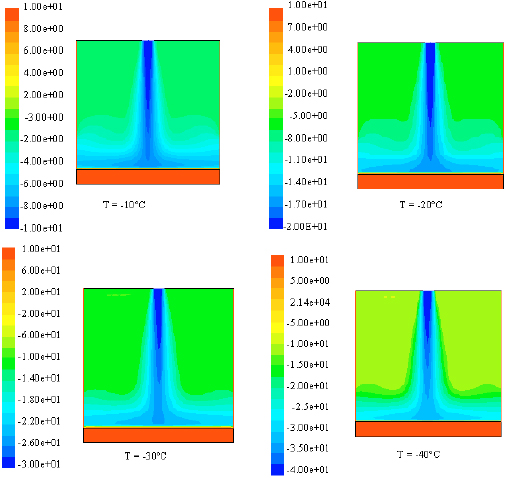 | |
| Fig. 6: | Effect of freezing air temperature on temperature distribution (°C) in the air domain for the H = 36 cm, Uj = 10 m sec–1 |
 | |
| Fig. 7: | Effect of freezing air velocity on freezing time |
When the food is positioned downstream of the potential core the freezing air velocity is degraded from its nozzle exit value, the energy of the jet decayed because of the turbulence in free jet region causing lower heat-transfer coefficient.
 | |
| Fig. 8: | Effect of freezing air velocity on h-value for H = 36 cm, Tj= -10°C |
Effect of nozzle to food distance on freezing time: The results of our study showed that as distance between nozzle exit and food surface decreases, freezing time increases. Figure 10 and 11 show influence of nozzle to food distance on flow pattern and on freezing time,respectively.
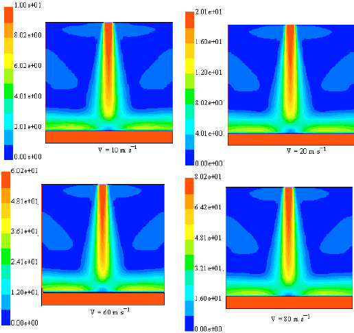 | |
| Fig. 9: | Effect of freezing air velocity on flow and velocity field for the H = 36 cm, Tj = -10°C |
Contours of velocity show that as the distance increases the flow has turbulent mixing characteristics before stagnation point and the potential core disappears completely. The presence of the potential core region results in lesser degree of vorticity at stagnation, causing a transition to turbulence in the wall region close to stagnation point. Longer distances result in actual turbulent dissipation and higher heat transfer coefficients at stagnation point but with an average low heat transfer coefficient. Further increasing the impinging distance results in a lack of fluid momentum to drive effective force convection, thus the thermal resistance increases. The appropriate distance increases with increasing Reynolds number of the impinging jet. Shorter distances can cause confinement, resulting in disturbance to the main jet streams. Our study shows that for food freezing applications nozzle-to-food distance ratio should be maintained in the range of 6-10. A wide range of experimental data on heat transfer measurements exists in this regard. Based on heat transfer measurements Gardon and Akfirat (1966) have suggested an optimal nozzle-to-food ratio of 6-8. The results on heat transfer coefficients and flow visualization studies indicated that heat transfer coefficients depended on nozzle-exit-to-food spacing. This is due to the turbulence induced at the boundary of the jet and the stagnant air. In many impingement applications, this type of turbulence tends to dissipate the energy in the jet region of the flow. To minimize energy dissipation, the nozzle-exit-to-plate spacing may be reduced, but an extremely short spacing between nozzle exit and the food causes unnecessary confinement of the jet. Confinement may prove advantageous in some cases but not so in others. In processing applications where moisture is being removed (baking, drying), confinement is not desirable, but in applications such as thawing, confinement may reduce drip loss by conserving moisture. When the food is positioned downstream of the potential core the freezing air velocity is degraded from its nozzle exit value, the energy of the jet decayed because of the turbulence in free jet region causing lower heat-transfer coefficient and the food is cooled ineffectively.
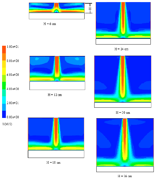 | |
| Fig. 10: | Effect of nozzle-to-food distance (H) on flow pattern for the Uj = 10 m sec–1, Tj= -10°C |
 | |
| Fig. 11: | Influence of nozzle to food distance on freezing time |
The nozzle-to-plate spacing should be optimized for best results, depending on the application. Such optimization would require predictive relationships for heat transfer coefficients based on the position and flow conditions. Figure 9 also shows the formation of boundary layer on the surface of the product at short distances away from stagnation. Although the boundary layer observed is only the hydrodynamic boundary layer and not a true representation of the thermal boundary layer, it is strongly correlated to the thermal boundary layer and results in a steep decline in heat transfer coefficients at short distances away from stagnation.
The heat transfer from a slot jet impinging on a slab shaped food has been studied using CFD (FLUENT6.0) simulations with Reynolds Stress turbulence (RSM) model. The CFD simulation results show how different impingement conditions (e.g., air velocity and temperature, nozzle to food distance) affect the freezing time of slab shaped foods and the information on these may be used in further optimization studies. The results of this study show that:
| • | Impinging air temperature is the most important variable, influencing freezing time. |
Lowering impinging air temperature, freezing time decreases but beyond critical point, it decreases slowly because the freezing air temperature showed little effect on the heat transfer coefficient.
| • | The velocity of the impinging air plays an important role in the thermal resistance. |
Increasing the velocity consistently diminishes the thermal resistance. Freezing time decreases with increasing impinging air velocity because convective heat transfer coefficient improves at higher velocities.
| • | The distance between the nozzle exit and the food is the other parameter affecting freezing time. Nozzle-to-food distances in the region of 6-8 are best because they ensure that the potential core is fully decayed and there is no excessive energy dissipation. |
These results indicate that with proper optimization of above mentioned parameters, major improvements can be achieved in air impingement food freezing systems.
ACKNOWLEDGMENTS
The corresponding author would like to thank to Mr. M. Mohammad pour Fard, Mechanical Engineering Ph.D. student of Mechanical Engineering Faculty, University of Tabriz for his valuable help during this study.
NOMENCLATURE
| Bj | = | Width of jet |
| d | = | Thickness of slab shaped food |
| H | = | Nozzle-to-food distance |
| h | = | Convective heat transfer coefficient |
| Cj | = | Specific heat of unfrozen food |
| Cs | = | Specific heat of frozen food |
| CP | = | Heat capacity at constant pressure |
| Cv | = | Heat capacity at constant volume |
| K | = | Thermal conductivity |
| kj | = | Thermal conductivity of unfrozen food |
| ks | = | Thermal conductivity of frozen food |
| L | = | Length of slab shaped food |
| Lf | = | Latent heat of freezing |
| P | = | Pressure |
| qv | = | Internal source term due freezing |
| T | = | Average temperature |
| Tf | = | Freezing temperature of food |
| Ti | = | Initial temperature of freezing food |
| Tj | = | Temperature of freezing air |
| T´ | = | Fluctuating component of temperature |
| t | = | Time |
| U | = | Average velocity |
| Uj | = | Velocity of air at nozzle exit |
| u´ | = | Turbulent component of velocity |
| ‹u´iu´j› | = | The average value of the fluctuating component of the velocity |
| X | = | Stream wise coordinate |
| Y | = | Coordinates perpendicular to stream wise coordinate direction |
| ρ | = | Density |
| γ | = | Kinematics viscosity of the air |
REFERENCES
- Borquez, R., W. Wolf, W.D. Koller and W.E.L. Speiss, 1999. Impinging jet drying of pressed fish cake. J. Food Eng., 40: 113-120.
CrossRefDirect Link - Campanone, A., V.O. Savadori and R.H. Mascheroni, 2005. Food freezing with simultaneous surface dehydration: Approximate prediction of weight loss during freezing and storage. Int. J. Heat Mass Transfer, 48: 1195-1204.
CrossRefDirect Link - Dagtekin, I. and H.F. Octopi, 2007. Heat transfer due to double laminar slot jets impingement on to an isothermal wall within one side closed long duct. Int. Commun. Heat Mass Transfer, 35: 65-75.
CrossRefDirect Link - Erdogdu, F., A. Sarkar and R.P. Singh, 2005. Mathematical modeling of air-impingement cooling of finite slab shaped objects and effect of spatial variation of heat transfer coefficient. J. Food Eng., 71: 287-294.
CrossRefDirect Link - Gardon, R. and J.C. Akfirat, 1966. Heat transfer characteristics of impinging two-dimensional air jets. J. Heat Trans., 88: 101-107.
CrossRefDirect Link - Huan, Z., S. He and Y. Ma, 2003. Numerical simulation and analysis for quick-frozen food processing. J. Food Eng., 60: 267-273.
CrossRefDirect Link - Lujan-Acosta, J., R.G. Moreira and J. Seyed-Yagoobi, 1997. Air-impingement drying of tortilla chips. Dry. Technol., 15: 881-897.
CrossRefDirect Link - Mittald, G.S. and J. Zhang, 2000. Prediction of freezing time for food products using a neural network. J. Food Res. Int., 33: 557-562.
CrossRefDirect Link - Moreira, R.G., 2001. Impingement drying of foods using hot air and superheated steam. J. Food Eng., 49: 291-295.
CrossRefDirect Link - Nitin, N. and M.V. Karwe, 2001. Heat transfer coefficient for cookie shaped objects in a hot air jet impingement oven. J. Food Process Eng., 24: 51-69.
Direct Link - Salvador, V.O. and R.H. Mascheroni, 2002. Analysis of impingement freezers performance. J. Food Eng., 54: 133-140.
CrossRefDirect Link - Sarkar, A. and R.P. Singh, 2004. Air impingement technology for food processing: Visualization studies. Lebensmittel-Wissehschaft und-Technologie, 37: 873-879.
Direct Link - Soto, V. and R. Borquez, 2001. Impingement jet freezing of biomaterials. J. Food Control, 12: 515-522.
CrossRefDirect Link - Wang, Z., H. Wu, G. Zhao, X. Liao, F. Chen, J. Wu and X. Hu, 2007. One-dimensional finite-difference modeling on temperature history and freezing time of individual food. J. Food Eng., 79: 502-510.
CrossRefDirect Link