
Ashok Sahai
Department of Statistics and Demography, University of Swaziland, Kwaluseni, P. Bag 4, Swaziland, Africa
M. Mahibbur Rahman
Department of Statistics and Demography, University of Swaziland, Kwaluseni, P. Bag 4, Swaziland, Africa
Rameshwar P. Jaju
Department of Computer Science,
University of Swaziland, Kwaluseni, P. Bag 4, Swaziland, Africa
Journal of Applied Sciences
Year: 2005 | Volume: 5 | Issue: 9 | Page No.: 1575-1581


ABSTRACT
Long-term data-sets of good quality are invaluable in certain research investigations. In some situation, they are so expensive of time and money, that they are seldom available. It has been noted that the problems of varying data quality, of missing information and that of diversity of data might possibly be dealt with by using meta-data. The key point is to treat relevant good quality meta-data as auxiliary/ancillary information, the use of which is gained through the proposed optimal simple estimation strategies. These strategies are motivated by mixing-type estimators, the desired optimality of these estimators is achieved through optimal manipulation of two design-parameters therein set to control first and second order of large sample approximations to their standard errors. A sensitivity analysis is then used to discover, empirically, the robust estimation strategy from amongst the proposed alternatives.
PDF Abstract XML References Citation
How to cite this article
Ashok Sahai, M. Mahibbur Rahman and Rameshwar P. Jaju, 2005. Using Meta-analysis for Data Enrichment-optimal Families of Estimation Strategies. Journal of Applied Sciences, 5: 1575-1581.
DOI: 10.3923/jas.2005.1575.1581
URL: https://scialert.net/abstract/?doi=jas.2005.1575.1581
DOI: 10.3923/jas.2005.1575.1581
URL: https://scialert.net/abstract/?doi=jas.2005.1575.1581
INTRODUCTION
Meta-analysis can be a useful tool in several research experiments where certain data are directly effected by natural events. The examples could include environmental research, forestry inventory control, sea food harvesting management, resource intensive or very costly natural experiments and other similar problems. For the purpose of our discussion, we have used the example of environmental research.
Many investigators, including Cuthbertson[1], have highlighted the value of meta-data and meta-analysis in environmental studies. For example, it is worth quoting from Hedges and Olkin[2]. “Finally, some notice might be in order regarding the usefulness of meta-analysis in environmental research. Using meta-analysis a researcher can ascertain which issues are likely to reward additional inquiry. In addition, at the peer-review level, which issues are likely to reward additional inquiry. In addition, at the peer-review level, meta-analysis can be used to synthesize apparently conflicting results into a unified corpus of knowledge”. Meta-analysis basically deals with techniques of synthesis of statistical inferences from two different/independent studies, possibly different spatially and/or at two different points of time. One of the currently investigated areas, receiving intensive attention of researchers in this field, is the handling of studies which might be dependent: possibly also with missing data[3,4].
From meta-data perspective, we would almost always have, at the meta-level, the temporal and spatial gaps in the data. Because of fast-changing environmental system-parameters in the present decade (by comparison with the years of, say, the preceding decade), time-series methods might not be adequate if we wish to have synthetic data for relevant system variables. On the contrary, using the preceding decade’s meta-data might well capture this fast-changing pattern more adeptly than the use of time series methods. It will, therefore, do better if treated via the use of ancillary/auxiliary variables setup, to capture this rather-faster-changing pattern more adeptly than via the time-series methods. In addition, there might be many spatial gaps where the underdeveloped and developing countries have insufficient resources, not enough to monitor many of the environmental system-variables, for some variables, data may not be available at all. To fill these gaps, small-scale surveys may be conducted by international agencies. However. Some of the variables may continue to be missing due to practical reasons, such as the lack of suitable infrastructure for the experimental work, etc.
Therefore, same strategy of using information on the ancillary/auxiliary variables would be appropriate for those missing variables. It is necessary to devise an estimation strategy which would exploit the high correlation (positive or negative) between the study variables and ancillary/ auxiliary variables. There are two main facts to be noted in this context: firstly, the usable data on such auxiliary/ancillary variables may not be extensive. The available data on such variables might have high dispersion temporally and/or spatially. Therefore it might not be advisable to use more than say, ten to twenty years’ data due to rapidly changing environmental system. Similarly in the other case, due to high spatial variability of data it could be equally undesirable to use data on the relevant auxiliary variable for more than ten or possibly less number of countries or sites with similar environmental zone where such a data becomes available. Secondly, due to system-dynamics of the environs and its rapidly changing patterns (spatially and temporally), the dispersion of the relevant meta-data on such an auxiliary/ancillary variables would be relatively very high. This has to be tackled statistically in as much as the variances of sub-groups (spatial/temporal) of data on such variables should not be highly significantly different to be synthesized in meta-data setup.
The data on the environmental variables are usually collected using small samples. Otherwise the data become very expensive. In some instances, if the study continues for longer period, the information on certain environmental variable becomes more expensive. Specially in the case of developing countries, it is very common to face the problem of missing information (spatial and/or temporal) on environmental variables due to limited availability of resources to monitor those. To overcome these difficulties, we might be better off is we tackle the gaps in the data using meta-data setup by searching for highly correlated (but relatively dispersed) variables having auxiliary/ancillary status of information for the study variable.
EXAMPLE APPLICATION
To illustrate, survey results for 19 landslide-damaged sites are reported by Reddy and Singh[5]. Eleven of these sites were in Oak-zone and 8 were in Pine or mixed Pine zones. Vegetation analysis was carried out for 10 one meter-squared quadrants: Biomass of the herb layer at the peak growth stage (i.e. in last week of august) was determined for 5 soil monoliths (25x25x30 cm (deep)) excavated randomly. Soil samples were collected in triplicate, from each site from 0-10 cm soil depths. Statistical analysis was done via the analysis of variance and non-linear regressions. We note that all the data were collected using small samples. Here the variable (age of site in years), say X, was found to be a good auxiliary variable. The relative dispersion for X was high: CX = 0.98 for Pine-zone and CX = 1.09 for Oak-zone: It was almost double of the relative dispersion of one of the important study variable, namely, A:P (Annual to Perennial (Herb-species) Ratio), say Y, with CY = 0.48 for the Pine-zone and CY = 0.57 for the Oak-zone. The corresponding values of CY for the other study variables for these two zones were (0.18, 0.28), (0.10, 0.19), (0.50, 0.42) and (0.62, 0.61); when Y ≡ Species, Annuals, Perennial and Cover, respectively and were as high as 0.81 and 0.90, when Y ≡ Density. Reddy and Singh[5] reported many couples of variables with a significantly high correlation: ± 0.6 to as high as 0.972. For the one relevant to our example, the coefficient of correlation between the study variables Y (i.e. A:P Ratio) and the auxiliary variables X (i.e. age of site) are fairly significant as reported in the paper: -0.718 for Pine-zone and –0.420 for Oak-zone.
Thus in the context of environmental database management in the meta-data setup and in the light of the aforesaid facts, we need to devise (for small sample) an estimation strategy for transporting the ancillary information, contained in as auxiliary variable (X). This variable X would be having a significant correlation with the study variable (Y); whereas, X-data might well be rather much more dispersed than the Y-data.
THE ESTIMATORS
The estimation strategies proposed in this study are motivated by the mixing-type estimation of Vos[6]. Sahai[7] used auxiliary information efficiently in his mixing type estimators. The same goal of efficiency is addressed here using auxiliary information (when the sample is small, i.e. n<30) for the problem of estimating the population average of the study variable. Subsequently, it can be used in aggregation or disaggregation of meta-data. In practice, it is possible to get hold of such an auxiliary variable with population mean (e.g. population average of age (in years) of the Oak-zone/Pine-zone sites in the proceeding illustration) which could either be known or could be know using past information.
With the above motivation, the following families of estimates are proposed. Each of these two families of estimates consists of two non-stochastic design parameters, namely α and β:
| (1) |
and
| (2) |
Where, x̄ and ![]() are the sample means of the auxiliary and study variables, respectively and is the population mean of auxiliary variable. The choice of the appropriate values for the two design-parameters is governed by their roles to minimize the first order approximation (upto the terms of O(n-1) and the second order approximation (upto terms O(n-2)) to the standard error of the relevant estimators. Further, the use of estimators in these families is highly recommended, provided the absolute value of the quantity within square brackets of Eq. 1 and 2 (i.e., the perturbators for
are the sample means of the auxiliary and study variables, respectively and is the population mean of auxiliary variable. The choice of the appropriate values for the two design-parameters is governed by their roles to minimize the first order approximation (upto the terms of O(n-1) and the second order approximation (upto terms O(n-2)) to the standard error of the relevant estimators. Further, the use of estimators in these families is highly recommended, provided the absolute value of the quantity within square brackets of Eq. 1 and 2 (i.e., the perturbators for ![]() ) stay away from unity on its either side by upto 30 percent of the quantity (1+2ρ2) where, ρ is the coefficient of correlation between the two variables X and Y. We may note that the term (1 + 2ρ2) is the leading multiplier of the second order approximation of the mean square error Eq. 10 and 11. The simulation study reported that only in 3% to 9% of the cases (depending on ρ values) the perturbations stay out of these bounds.
) stay away from unity on its either side by upto 30 percent of the quantity (1+2ρ2) where, ρ is the coefficient of correlation between the two variables X and Y. We may note that the term (1 + 2ρ2) is the leading multiplier of the second order approximation of the mean square error Eq. 10 and 11. The simulation study reported that only in 3% to 9% of the cases (depending on ρ values) the perturbations stay out of these bounds.
It may be noted that the mixing estimators of Vos[6] are:
| (3) |
and
| (4) |
wherein ![]() are the well-known product and quotient estimators, respectively and α is the design-parameter that minimizes the first order approximation (O(n-1)) to the standard error of the estimator.
are the well-known product and quotient estimators, respectively and α is the design-parameter that minimizes the first order approximation (O(n-1)) to the standard error of the estimator.
On the other hand structurally, the proposed families of estimators happen to be a result of marrying the perspective of the one-parameter, family of the estimators, ![]() sa [7] and the one with that of
sa [7] and the one with that of ![]() [8]. These are, respectively:
[8]. These are, respectively:
| (5) |
| (6) |
where, in both cases the value of the design-paramater, α is chosen similarly as in the case of the estimators of Vos[6], so that it minimizes the first order approximation (O(n-1)) to the standard error of the respective estimators. It is worth noting that the proposed families of estimators inherit the perspective of a version of ![]() sr [8] and that a fractional α is not computationally favorable to numerical exponential approximation. Another such estimator with a similar perspective has been given by Reddy[9]:
sr [8] and that a fractional α is not computationally favorable to numerical exponential approximation. Another such estimator with a similar perspective has been given by Reddy[9]:
| (7) |
Note that the above estimator is embedded in the proposed family of estimators ![]() αβ (1) with α = 0, i.e. one-parameter sub-family without the facility of exploitation of a second degree of freedom. Then, the only parameter β controls both first and second order of approximations to the mean square error.
αβ (1) with α = 0, i.e. one-parameter sub-family without the facility of exploitation of a second degree of freedom. Then, the only parameter β controls both first and second order of approximations to the mean square error.
Using the result of bivariate normal population[10], we get the following expressions for the first and second order of approximations to the Mean Square Error (MSE) of the relevant estimators (MSE1(.) and MSE2(.)), respectively
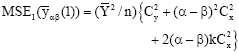 | (8) |
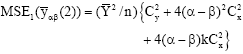 | (9) |
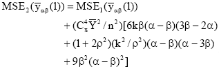 | (10) |
and
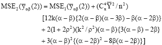 | (11) |
where, k = ρ(Cy/Cz). By minimizing MSE1(.) and MSE2(.) in Eqs. 8 to 11, we get:
| (12) |
| (13) |
To use these optimal values of design-parameters, we are constrained by the lack of knowledge of the values of ρ and k, where k is a function of ρ and Cy/Cx (Eq.12 and 13). However, we use the easily available close guesses on ρ and Cy/Cx via the past data or long association with the experimental setup in order to obtain a value for k.
To study the sensitivity (robustness) of the estimators in the proposed families to the relative errors in guessing k as also to study their relative efficiencies in order to discover the appropriate estimation strategy to be recommended in a practical situation, an extensive simulation study was carried out.
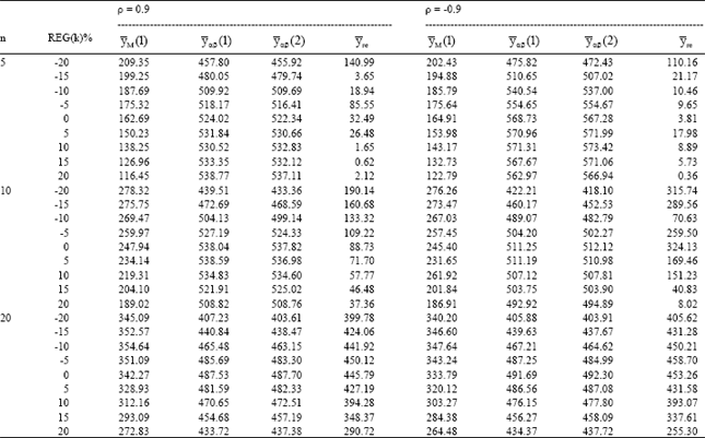
| Table 1: | Relative efficiency for different ratio-product estimators |
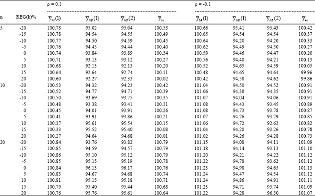 | |
| Table 2: | Relative efficiency for different ratio-product estimators |
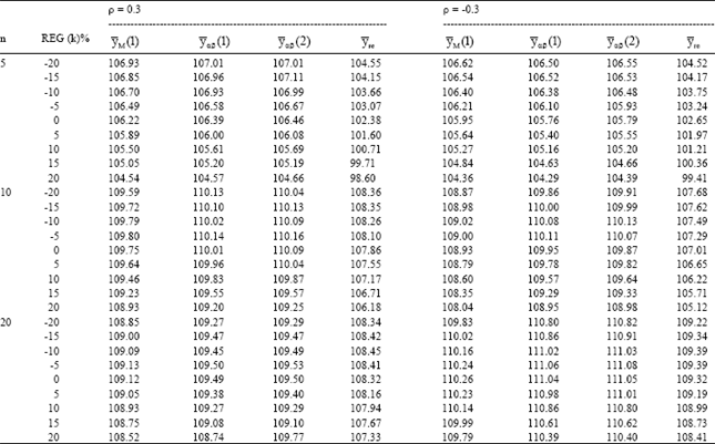 | |
| Table 3: | Relative efficiency for different ratio-product estimators |
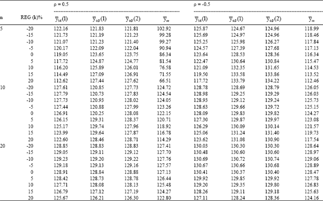 | |
| Table 4: | Relative efficiency for different ratio-product estimators |
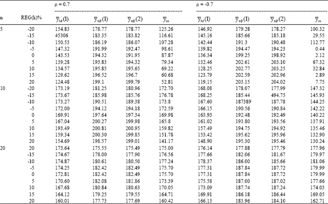 | |
| Table 5: | Relative efficiency for different ratio-product estimators |
 | |
RESULTS AND DISCUSSION
For simulation study, we consider two independent normal populations with
μY = 6, σY = 6 and μX = 6, σX = 12 so that CX = 2CY
We generate respective bivariate normal population using ten different values: ±0.1, ±0.3, ±0.5, ±0.7 and ±0.9 for three different sample sizes: n = 5, 10 and 20.
Also to discover the robustness of the estimators (1) and (2), we carry out sensitivity analysis using nine cases of the relative error in guessing k by using g, say -
REG(k) = [(g-k)/k]100%
We have generated 5000 samples for each combination of n, ρ and REG(k) and have calculated the actual MSE of all the estimators mentioned (Eqs. 1 to 7). These results are summarized in Table 1-5. The tabulated values represent the relative efficiencies of the estimators.
![]()
Table 1-5 are organized for different data of coefficient of correlation-(ρ), sample size (n) and REG (k) = 0, ±5%, ±10%, ±15% and ±20%.
The results are encouraging for the proposed families of estimators. As expected, ![]() sa and
sa and ![]() sr din not perform so well as the estimators of the proposed families. The same happened to Vos’[6]
sr din not perform so well as the estimators of the proposed families. The same happened to Vos’[6] ![]() M (2) as compared to his
M (2) as compared to his ![]() M(1). Hence we excluded these estimators while presenting these results.
M(1). Hence we excluded these estimators while presenting these results.
The results also shows that:
| • | For |ρ| ≥ 0.5, the proposed families of estimators are significantly more efficient as compared to |
| • | When the correlation is very low (say |ρ| < 0.3), the estimators |
| • | In the case to under-guess (i.e. when REG(k) is negative), |
| • | For the case of the over-guess (i.e. when REG(k) is positive), |
Therefore, in practice, it will be prudent to use the estimation strategy via the simple mixing:
since it would be unknown to us as to whether we are under-guessing of over-guessing.