
A. Prabhu Britto
Center for Medical Electronics, Department of Electronics and Communication Engineering, Anna University, Chennai 600025, India
G. Ravindran
Faculty of Information and Communication Engineering, Anna University, Chennai 600025, India
Information Technology Journal
Year: 2007 | Volume: 6 | Issue: 3 | Page No.: 441-447


ABSTRACT
This research analyses Discrete Cosine Transform based Gradient Vector Flow Active Contours, a segmentation tool for chromosome spread images, which have hitherto been established as an efficient segmentation tool. Extensive research has been performed on Discrete Cosine Transform based Gradient Vector Flow Active Contours for segmentation of chromosome spread images. This study is an extended analysis in the same area. This study yields more insight on efficient segmentation of chromosome spread images using Discrete Cosine Transform based Gradient Vector Flow Active Contours.
PDF Abstract XML References Citation
How to cite this article
A. Prabhu Britto and G. Ravindran, 2007. Discrete Cosine Transform Based Gradient Vector Flow Active Contours for Chromosome Image Segmentation-an Analysis. Information Technology Journal, 6: 441-447.
DOI: 10.3923/itj.2007.441.447
URL: https://scialert.net/abstract/?doi=itj.2007.441.447
DOI: 10.3923/itj.2007.441.447
URL: https://scialert.net/abstract/?doi=itj.2007.441.447
INTRODUCTION
Active contours are used extensively in computer vision and image processing applications, particularly to locate object boundaries. The main advantage of Active Contours is the ability to generate closed parametric curves from images. Problems associated with initialization and poor convergence to concave boundaries, however, have limited their utility. To overcome these difficulties in initialization and poor convergence to object boundaries, a new external force model was suggested that used a convex combination of the usual external force and a new force derived from an estimate of the local curvature of the object boundary. This force simultaneously pulled the snake toward the boundary and into the concave region (Prince and Xu, 1996). This was later improved by Xu and Prince (1998) to form the Gradient Vector Flow (GVF) field. The resulting formulation produces external force fields that had both irrotational and solenoidal components (Xu and Prince, 1998), which had a large capture range overcoming the difficulty associated with initialization of Active Contours and it was also able to provide good convergence to concave boundaries. Tang and Acton (2004) have given an improved form of the GVF field, called the Discrete Cosine Transform (DCT) based GVF. The authors have performed extensive experimentation and analysis on the chromosome spread image segmentation performance of DCT based GVF Active Contours (Britto and Ravindran, 2005a,b, 2006a-d). This study, analysed the segmentation obtained using Discrete Cosine Transform based Gradient Vector Flow Active Contours in chromosome spread images, which have hitherto been established as an efficient segmentation tool for chromosome spread images.
ACTIVE CONTOUR MODELS
Active Contours also called as Snakes or Deformable Curves, first proposed by Kass et al. (1987) are energy minimizing contours that apply information about the boundaries as part of an optimization procedure. They are generally initialized by automatic or manual process around the object of interest. The contour then deforms itself iteratively from its initial position in conformity with the nearest dominant edge feature, by minimizing the energy composed of the Internal and External forces, converging to the boundary of the object of interest. The Internal forces computed from within the Active Contour enforce smoothness of the curve and External forces that are derived from the image help to drive the curve toward the desired features of interest during the course of the iterative process.
The energy minimization process can be viewed as a dynamic problem where the active contour model is governed by the laws of elasticity and lagrangian dynamics (Rueckert, 1997) and the model evolves until equilibrium of all forces is reached, which is equivalent to a minimum of the energy function. The energy function is thus minimized, making the model active.
FORMULATION OF ACTIVE CONTOUR MODELS
An Active Contour Model can be represented by a curve c, as a function of its arc length τ,
(1) |
with τ = [0...1]. To define a closed curve, c(0) is set to equal c(1). A discrete model can be expressed as an ordered set of n vertices as vi = (xi,yi)T with v = (v1,...,vn). The large number of vertices required to achieve any predetermined accuracy could lead to high computational complexity and numerical instability (Rueckert, 1997).
Mathematically, an active contour model can be defined in discrete form as a curve ![]() that moves through the spatial domain of an image to minimize the energy functional
that moves through the spatial domain of an image to minimize the energy functional
 | (2) |
where α and β are weighting parameters that control the active contour’s tension and rigidity respectively (Xu and Prince, 1997). The first order derivative discourages stretching while the second order derivative discourages bending. The weighting parameters of tension and rigidity govern the effect of the derivatives on the snake.
The external energy function Eext is derived from the image so that it takes on smaller values at the features of interest such as boundaries and guides the active contour towards the boundaries. The external energy is defined by
(3) |
where, Gσ(x,y) is a two-dimensional Gaussian function with standard deviation σ, I(x,y) represents the image and κ is the external force weight. This external energy is specified for a line drawing (black on white) and positive κ is used. A motivation for applying some Gaussian filtering to the underlying image is to reduce noise. An active contour that minimizes E must satisfy the Euler Equation
(4) |
where Fint = αx”(s)-βx”“(x) and Fext = -∇Eext comprise the components of a force balance equation such that
Fint+Fext = 0 | (5) |
The internal force Fint discourages stretching and bending while the external potential force Fext drives the active contour towards the desired image boundary. Equation (4) is solved by making the active contour dynamic by treating x as a function of time t as well as s. Then the partial derivative of x with respect to t is then set equal to the left hand side of Eq. (4) as follows
(6) |
A solution to Eq. (6) can be obtained by discretizing the equation and solving the discrete system iteratively (Kass et al., 1987). When the solution x(s,t) stabilizes, the term xt(s,t) vanishes and a solution of Eq. (4) is achieved.
Traditional active contour models suffer from a few drawbacks. Boundary concavities leave the contour split across the boundary. Capture range is also limited. Hence a new external force was developed (Prince and Xu, 1996). Three guiding principles led to the development of the new external force. The first aim was the ability to add the new force to the existing force. Since the existing force was the gradient of a scalar function (the energy Eext), it was an irrotational (curl-free field). According to the Helmholtz theorem, the other fundamental field component was a solenoidal (divergence-free) field. Therefore, the new field was chosen to be solenoidal. The second aim was that the new field should not disturb the equilibrium contours of the external energy in the absence of internal forces. Therefore, the new field should be zero whenever the field -∇Eext is zero. The third aim wanted the field to point toward the apex of concave boundary regions, a feature defined by the object boundary curvature. Therefore, the new field was made to use a measure of boundary curvature in its definition (Prince and Xu, 1996). This was later improved by Xu and Prince (1997) to form the Gradient Vector Flow (GVF) field. Xu and Prince (1997) presented a new external force, called Gradient Vector Flow (GVF), which was computed as a diffusion of the gradient vectors of a gray-level or binary edge map derived from the image. The resultant field had a large capture range and forces the active contours into concave regions (Xu and Prince, 1998, 2000).
The overall approach was to define a new non-irrotational external force field, called as the GVF field. The earlier idea of constructing a separate solenoidal field from an image and adding it to a standard irrotational field was improved and a more natural approach was designed in which the external force field is designed to have the desired properties of both large capture range and presence of forces that point into boundary concavities. The resulting formulation produces external force fields that had both irrotational and solenoidal components (Xu and Prince, 1998).
GRADIENT VECTOR FLOW (GVF) ACTIVE CONTOURS
Gradient Vector Flow (GVF) Active Contours use Gradient Vector Flow fields obtained by solving a vector diffusion equation that diffuses the gradient vectors of a gray-level edge map computed from the image. The GVF active contour model cannot be written as the negative gradient of a potential function. Hence it is directly specified from a dynamic force equation, instead of the standard energy minimization network. The external forces arising out of GVF fields are non-conservative forces as they cannot be written as gradients of scalar potential functions. The usage of non-conservative forces as external forces show improved performance of Gradient Vector Flow field Active Contours compared to traditional energy minimizing active contours (Xu and Prince, 1998, 2000).
The GVF field points towards the object boundary when very near to the boundary, but varies smoothly over homogeneous image regions extending to the image border. Hence the GVF field can capture an active contour from long range from either side of the object boundary and can force it into the object boundary. The GVF active contour model thus has a large capture range and is insensitive to the initialization of the contour. Hence the contour initialization is flexible.
The gradient vectors are normal to the boundary surface but by combining Laplacian and Gradient the result is not the normal vectors to the boundary surface. As a result of this, the GVF field yields vectors that point into boundary concavities so that the active contour is driven through the concavities. Information regarding whether the initial contour should expand or contract need not be given to the GVF active contour model. The GVF is very useful when there are boundary gaps, because it preserves the perceptual edge property of active contours (Kass et al. 1987; Xu and Prince, 1998). The GVF field is defined as the equilibrium solution to the following vector diffusion equation (Xu and Prince, 2000),
(7a) |
(7b) |
where, ut denotes the partial derivative of u(x,t) with respect to t, ∇2 is the Laplacian operator (applied to each spatial component of u separately) and f is an edge map that has a higher value at the desired object boundary. The functions in g and h control the amount of diffusion in GVF. In Eq.(7), g(|∇f|)∇2u produces a smoothly varying vector field and hence called as the smoothing term, while h(|∇f|)(u-∇f) encourages the vector field u to be close to ∇f computed from the image data and hence called as the data term. The weighting functions g(·) and h(·) apply to the smoothing and data terms, respectively and they are chosen15 as g(|∇f|) = μ and h(|∇f|) = |∇f|2. g(·) is constant here and smoothing occurs everywhere, while h(·) grows larger near strong edges and dominates at boundaries. Hence, the Gradient Vector Flow field is defined as the vector field v(x, y) = [u(x, y), v(x, y)] that minimizes the energy functional
(8) |
The effect of this variational formulation is that the result is made smooth when there is no data.
When the gradient of the edge map is large, it keeps the external field nearly equal to the gradient, but keeps field to be slowly varying in homogeneous regions where the gradient of the edge map is small, i.e., the gradient of an edge map ∇f has vectors point toward the edges, which are normal to the edges at the edges and have magnitudes only in the immediate vicinity of the edges and in homogeneous regions ∇f is nearly zero. μ is a regularization parameter that governs the tradeoff between the first and the second term in the integrand in Eq. (8). The solution of Eq. (8) can be done using the Calculus of Variations and further by treating u and v as functions of time, solving them as generalized diffusion equations (Xu and Prince, 1998).
DISCRETE COSINE TRANSFORM (DCT) BASED GVF ACTIVE CONTOURS
The transform of an Image yields more insight into the properties of the image. The Discrete Cosine Transform has excellent energy compaction. Hence, the Discrete Cosine Transform promises better description of the image properties. The Discrete Cosine Transform is embedded into the GVF Active Contours. When the image property description is significantly low, this helps the contour model to give significantly better performance by utilizing the energy compaction property of the DCT.
The 2D DCT is defined as
 | (11) |
The local contrast of the Image at the given pixel location (k,l) is given by
 | (12) |
where,
 | (13) |
and
(14) |
Here, wt denotes the weights used to select the DCT coefficients. The local contrast P(k,l) is then used to generate a DCT contrast enhanced Image (Tang and Acton, 2004), which is then subject to selective segmentation by the energy compact gradient vector flow active contour model using Eq. (8).
RESULTS AND DISCUSSION
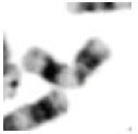
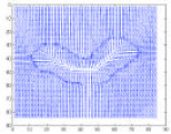
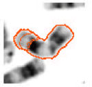
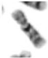
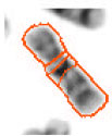
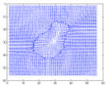
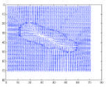
The characterized standardized parameters (Britto and Ravindran, 2005b, 2006a) of the DCT based GVF Active Contours are used in the DCT based GVF Active Contour formulation that was used to segment the chromosome spread images obtained from the Genomic Centre for Cancer Research and Diagnosis (GCCRD). The segmentation was successful without any preprocessing or enhancement procedures. Therefore no preprocessing or enhancement techniques was implemented on the images obtained from the GCCRD unlike the images that were obtained from other sources that required limited preprocessing and enhancement techniques to be implemented prior to segmentation using DCT based GVF Active Contours. A few graphical results are shown Fig. 1-5.
From Table 1, we find that the maximum absolute error along the major axis is 2.333239 pixels, while the minimum absolute error along the major axis is 0.923222 pixels. The maximum absolute error along the minor axis is 2.072397 pixels, while the minimum absolute error along the minor axis is 0.472095 pixels.
 | |
| Fig. 1a: | Sample 1 |
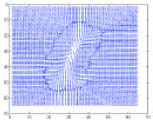 | |
| Fig. 1b: | DCT GVF field |
 | |
| Fig. 1c: | Segmented sample 1 |
 | |
| Fig. 2a: | Sample 2 |
 | |
| Fig. 2b: | DCT GVF field |
 | |
| Fig. 2c: | Segmented sample 2 |
 | |
| Fig 3a: | Sample 3 |
 | |
| Fig. 3b: | DCT GVF field |
 | |
| Fig. 3c: | Segmented sample 3 |
 | |
| Fig. 4a: | Sample 4 |
 | |
| Fig. 4b: | DCT GVF field |
 | |
| Fig. 4c: | Segmented sample 4 |
 | |
| Fig. 5a: | Sample 4 |
 | |
| Fig. 5b: | DCT GVF field |
 | |
| Fig. 5c: | Segmented sample 5 |
| Table 1: | Segmentation Error (GCCRD dataset) |
 | |
The statistics obtained earlier (Britto and Ravindran, 2006d) are as follows. From Britto and Ravindran (2006d) we find that the maximum absolute error along the major axis is 1.963482 pixels, while the minimum absolute error along the major axis is 0.055934 pixels. The maximum absolute error along the minor axis is 1.867320 pixels, while the minimum absolute error along the minor axis is 0.421066 pixels.
The contour thickness is 1 pixel wide and the contour iteration step size is 1 pixel. The difference between the respective statistics obtained now and earlier (Britto and Ravindran, 2006d) corroborates, as the difference between them is less than 1 pixel, which implies that the performance of the DCT based GVF Active Contours now and earlier has been the similar as they have converged with approximate similar error measures.
But the difference is that preprocessing and enhancement had been applied prior to segmentation earlier (Britto and Ravindran, 2006d), whereas no preprocessing and enhancement has been applied prior to segmentation now.
This implies that the DCT based GVF Active Contours may be a robust segmentation technique that may need neither preprocessing nor enhancement prior to segmentation.
If this inference is established, it will make the DCT based GVF Active Contour as a robust efficient segmentation technique.
ACKNOWLEDGMENT
The authors express their thanks to Dr. Michael Difilippantonio (Staff Scientist at the Section of Cancer Genomics, Genetics Branch/CCR/NCI/NIH, Bethesda MD); Prof. Ekaterina Detcheva (Artificial Intelligence Department, Institute of Mathematics and Informatics, Sofia, Bulgaria); Prof. Ken Castleman and Prof. Qiang Wu (Advanced Digital Imaging Research, Texas); Wisconsin State Laboratory of Hygiene (http://worms.zoology.wisc. edu/zooweb/Phelps/karyotype.html) and the Genomic Centre for Cancer Research and Diagnosis (GCCRD) (http://www.umanitoba.ca/institutes/manitoba_institute_cell_biology/GCCRD/GCCRD_Homepage.html) for providing chromosome spread images.
REFERENCES
- Britto, A.P. and G. Ravindran, 2005. A review of deformable curves from the perspective of chromosome image segmentation. J. Med. Sci., 5: 363-370.
CrossRefDirect Link - Britto, A.P. and G. Ravindran, 2005. Comparison of boundary mapping efficiency of gradient vector flow active contours and their variants on chromosome spread images. J. Applied Sci., 5: 1452-1460.
CrossRefDirect Link - Britto, A.P. and G. Ravindran, 2006. Boundary mapping of chromosome spread images using optimal set of parameter values in discrete cosine transform based gradient vector flow active contours. J. Applied Sci., 6: 1351-1361.
CrossRefDirect Link - Britto, A.P. and G. Ravindran, 2006. Detection of specific human chromosomal abnormalities using discrete cosine transform based gradient vector flow active contours. Biotechnology, 6: 111-117.
CrossRefDirect Link - Britto, A.P. and G. Ravindran, 2006. Evaluation of standardization of curve evolution based boundary mapping technique for chromosome spread images. Inform. Technol. J., 5: 94-107.
CrossRefDirect Link - Britto, A.P. and G. Ravindran, 2006. Segmentation of chromosome spread images using discrete cosine transform based gradient vector flow active contours: An analysis. J. Med. Sci., 6: 117-124.
CrossRefDirect Link - Kass, M., A. Witkin and D. Terzopoulos, 1988. Snakes: Active contour models. Int. J. Comput. Vision, 1: 321-331.
CrossRefDirect Link - Xu, C. and J.L. Prince, 1997. Gradient vector flow: A new external force for snakes. Proceedings of the IEEE Conference on Computer Vision and Pattern Recognition, June 17-19, 1997, San Juan, Puerto Rico, pp: 66-71.
CrossRef - Xu, C. and J.L. Prince, 1998. Snakes, shapes and gradient vector flow. IEEE Trans. Image Process., 7: 359-369.
CrossRefDirect Link