ABSTRACT
In this research, our objective is to evaluate the probability density function of z = xαyβ, where, x and y are two independent random variables, by using the probabilistic transformation method. The Probabilistic Transformation Methods (PTM) evaluate the Probability Density Function (PDF) of a function by multiplying the input pdf by the Jacobian of the inverse function. A new theorem for two input and one output has been developed. The result of our method is verified by the Monte Carlo simulation.
PDF Abstract XML References Citation
How to cite this article
DOI: 10.3923/ijaef.2007.105.112
URL: https://scialert.net/abstract/?doi=ijaef.2007.105.112
INTRODUCTION
A Random Equation (RE) is an equation containing a random term. The study of RE is an exciting topic which brings together techniques from probability theory, functional analysis and the theory of equations analysis.
Differential equations appear in several different applications: study of random evolution of systems with a spatial extension (random interface growth, random evolution of surfaces, fluids subject to random forcing), study of stochastic models where the state variable is infinite dimensional (for example, a curve or surface).
The solution to random equations may be viewed in several manners. We can view a solution as a random field (set of random variables indexed by a multidimensional parameter). In the case where the RE is an evolution equation, the finite dimensional points of view consists in viewing the solution at a given time as a random element in a space function and thus view the RE as a stochastic evolution equation in an infinite dimensional space. In the path wise point of view, tries to give a meaning to the solution for (almost) every realization of the noise and then view the solution as a random variable on the set of (infinite dimensional) paths thus defined.
The solution of a stochastic equation is gotten when we evaluate the probability density function of this solution. We can use several numerical methods, for example Fokker-Planck equation (Wojtkiewicz and Bergman, 2000), development of Wiener-Hermit (Hou and Wetton, 1992), method of perturbation (Falsone and Impollinia, 2002), method of stochastic local linearization (Jimenez et al., 1999), method of decomposition (Champier, 2000), stochastic finite element method (Sudret et al., 2004) and other.
In this research, a new technique is proposed in order to evaluate the probability density function of the solution, based on the combination of a known probabilistic transformation methods and a developed nonlinear technique.
The main disadvantage of the previous methods is that they are approximate methods and they are applicable under some conditions (e.g., the randomness should be small) as opposed the our developed method which is exact and applicable without any conditions.
PROBABILISTIC TRANSFORMATION METHOD
The Probabilistic Transformation Method is based on one-to-one mapping between the random output(s) and input(s) where the transformation Jacobian J can be computed. The pdf of the output(s) is then computed through the known joint pdf of the inputs multiplied by the determinant of transformation Jacobean matrix. The one-to-one mapping condition can be relaxed through some mathematical tricks (Kadry and Younes, 2005). The theory of the PTM is based on the following theorem (Freund et al., 2004):
Theorem 1
Suppose that X is a continuous random variable with pdf fx(x) and A⊂U is the one-dimensional space where, fX(x)>0, is differentiable and monotonic. Consider the random variable Y = u(X), where, y = u(x) defines a one-to-one transformation that maps the set A onto a set B⊂U so that the equation y = u(x) can be uniquely solved for x in terms of y, say x = u-1(y). Then, the pdf of Y is (Fig. 1):
| (1) |
Where:
| (2) |
is the transformation Jacobean, which must be continuous for all points y ∈ B.
We notice in the previous theorem that the function u(.) should be monotonic. For the general case of non monotonic functions, the following theorem allows us to consider a piecewise monotonic transformation.
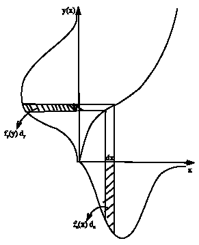 | |
| Fig. 1: | Transformation method |
Theorem 2
(pdf of piecewise monotonic transformation)
Let X be a continuous random variable with pdf fX(x) and Y = u(X) be a transformation of X. If there exists a partition A0,..., AK of A ⊂ R and functions u1(x),...uk (x) such that:
| • | P(X ∈ A0) = 0 |
| • | Each Ai for i ∈ {1,2,...,k} is an interval [ai, bi] (the endpoints are irrelevant, they can always be placed in A0. It is possible for ai to tend to -∞ and for bi to tend to ∞. |
| • | u(x) = ui(x) for all x ∈ Ai. |
| • | ui(x) is monotonic on each Ai. |
| • | ui(x) is differentiable over Ai. |
Then
| (3) |
The proof of this theorem can be found in (Hogg and Craig, 1994).
EXTENSIONS OF THE PTM
The common mathematical condition in all previous theorems is that the transformation must be one-to-one. A problem arises frequently when we wish to find the probability distribution of the random function Y = u(X) when X is a continuous random variable and the transformation is not one-to-one. This is usually the case of finite element analysis, where the interest is often focused on only one output variable (maximum stress or displacement), in terms of several input random variables.
In general, the two major limitations of the PTM are:
| • | The transformation function u(x) should be bijective. |
| • | The determinant of the Jacobean should be not nil. |
These two limitations can be avoided by suitable definition of the transformation problem, where additional output variables are added to ensure an equivalent one-to-one transformation.
In the case where we have only one output variable as a function of n input variables, we can proceed as following:
 | (4) |
Theorem 3 (Kadry and Younes, 2005)
The function U (above) is reversible, i.e., U-1 ∃.
Proof
The function u (above) is reversible if and only if the determinant of the Jacobean is not null. Indeed:
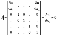 . At least, it exist i as . At least, it exist i as |
NONLINEAR TECHNIQUE
In practice, the problem of nonlinearity in the stochastic equation has been always faced; The difficulty arises when the nonlinear element is random. The proposed method in this situation is to substitute the element of the equation by using Variable Changes Technique which in turn allows us to apply the PTM. Let us consider the following stochastic equation:
| (5) |
Where, x and y are two independent random variables. Two principal cases are considered:
α > 0 |
In this case, the nonlinearity present in the numerator of the equation, i.e., x is random and α≥1. It requires linearizing the numerator, to do that we suppose δ = xa then by applying the PTM technique the pdf of δ,
| (6) |
α < 0 |
In this case, the nonlinearity appears in the denominator of the Stiffness Matrix Term, i.e., x is random and α ≤ -1. It requires linearizing the denominator, to do that we suppose δ = 1/xα then we apply the PTM technique to get the pdf of δ,
 | (7) |
Once the linearization step has been done, it’s required to find the pdf of the product of two random variables. To do that, we developed the following theorem:
Theorem 4
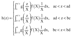
Let X be a continuous random variable with PDF f(X) which is defined and positive on the interval [a, b], where, 0<a<b<∞. Similarly, let Y be a random variable of the continuous type with PDF g(Y) which is defined and positive on the interval [c, d], where, 0<c<d<∞. The PDF of z = XY, h(z), is:
Case: ad<bc
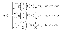 |
Case 2: ad = bc
 |
Case 3: ad>bc
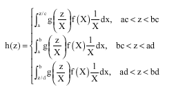 |
Proof
Only the case of ad<bc is considered. The other cases are proven analogously. Using Theorem 1 and Theorem 3, the transformation w = X and z = XY is bijective. The Jacobian of this transformation become:
 |
The joint PDF of w and z is:
| (8) |
Integrating with respect to w over the appropriate intervals and replacing w with X in the final result yields the marginal PDF of z:
 |
as desired.
APPLICATIONS
| • | Let us consider in the first application the following stochastic equation: z = xy, where, x and y are two independent random variables. For example x is uniformly distributed on the range of [1,2] and y is uniformly distributed on the range of [3,4] (Fig. 2). i.e., |
Using Theorem 3, the pdf of z (z = xy) become (Fig. 3):
 |
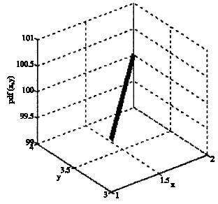 | |
| Fig. 2: | Joint pdf of x and y |
 | |
| Fig. 3: | pdf (z = xy) where, x→U(1,2) and y→U(3,4) |
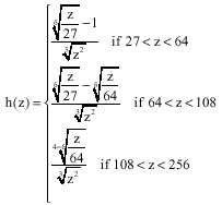
| • | In the second application, we studied the following stochastic equation: z = x2y3, where, x and y are two independent random variables. For example x is uniformly distributed on the range of [1,2] and y is uniformly distributed on the range of [3,4] (Fig. 4). Let us suppose X = x2 and Y = y3, by using the nonlinearity technique (see §IV): |
 |
and
 |
Using Theorem 3, the pdf of z (z = x2y3) become (Fig. 5):
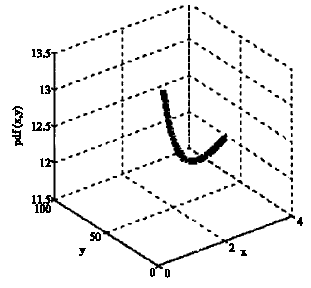 | |
| Fig. 4: | Joint pdf(X,Y) |
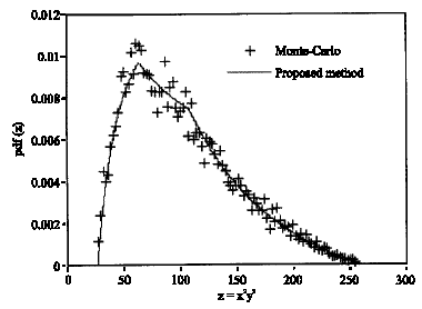 | |
| Fig. 5: | pdf(z = x2y3) where, x→U(1,2) and y→U(3,4) |
 |
CONCLUSION
In this study, an effective technique, based on the probabilistic transformation method, to calculate the probability density function of the product of two nonlinear independent random variables has been developed. The accuracy of this technique is validate by Monte-Carlo simulations.
REFERENCES
- Falsone, G. and N. Impollonia, 2002. A new approach for the stochastic analysis of finite element modelled structures with uncertain parameters. Comput. Methods Applied Mech. Eng., 191: 5067-5085.
CrossRef - Jimenez, J.C., I. Shoji and T. Ozaki, 1999. Simulation of stochastic differential equations through the local linearization method. J. Stat. Phys., 94: 587-602.
CrossRefDirect Link


