
O. E. Okereke
Department of Maths, Statistics and Computer Science, Michael Okpara University of Agriculture, Umudike, Nigeria
Asian Journal of Mathematics & Statistics
Year: 2011 | Volume: 4 | Issue: 4 | Page No.: 181-185


ABSTRACT
This study improves on the alternative method of obtaining least squares estimates of the parameters of a simple linear regression model by virtue of adding constant to at least one of the associated variables. It is observed that the estimate of the slope is not affected by addition of a constant to any or both of the variables. The estimate of the intercept is a function of the added constant(s). The relationships between the several intercepts of those models involving the transformed values of the variables and that of the original model are then obtained so to facilitate comparison and referencing. These theoretically obtained results have been validated with the help of empirical data analysis.
PDF Abstract XML References Citation
Received: March 23, 2011;
Accepted: May 04, 2011;
Published: July 05, 2011
How to cite this article
O. E. Okereke, 2011. Some Consequences of Adding a Constant to at Least One of the Variables in the Simple Linear Regression Model. Asian Journal of Mathematics & Statistics, 4: 181-185.
DOI: 10.3923/ajms.2011.181.185
URL: https://scialert.net/abstract/?doi=ajms.2011.181.185
DOI: 10.3923/ajms.2011.181.185
URL: https://scialert.net/abstract/?doi=ajms.2011.181.185
INTRODUCTION
Regression analysis is one of the most commonly used statistical tools (Ding, 2006; El-Salam, 2011). It has been found useful in describing the relationship which exists between variables and forecasting the value of a dependent variable corresponding to a given value(s) of the independent variable(s). No doubt, the knowledge of the future values of the dependent variable obtained through forecasting helps organizations, companies and governments in the area of policy and decision making. As a result, this statistical method has gained the attention of researchers and practitioners in various fields of study. Rajarathinam and Parmar (2011) developed a statistical model to fit the trends in area, production and productivity of castor crop based on both parametric and non-parametric regression models and to estimate growth rates. Consumer preferences for a soft drink have been studied using factor analysis (Abdullah and Asngari, 2011). Igwenagu (2011) in the study of CO2 emission discovered that gross domestic product and industrial output accounted for 93% of the total variation. El-Shehawy (2008) presented computational tools in S-plus based on cross-validation and bootstrapping for the adequate selection of the parametric models such as non-linear regression models (NRL-Models).
Consider a simple linear regression model specified as:
| (1) |
The least square estimates of α and β denoted by a and b respectively are given as:
| (2) |
and:
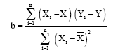 | (3) |
This least squares method is aimed at minimizing the sum of squared errors between the observed values of the dependent variable and the values that would be fitted under the assumed relationship (Nwabuokei, 1986). Least squares estimation of parameters of the model in Eq. 1 is usually based on certain assumptions. The errors are assumed to be from a single population with zero mean and constant variance (Steel and Torrie, 1981). Olaomi and Ifederu (2008) also pointed out there is lack of autocorrelation of error terms and the zero covariance between the explanatory variable and error terms.
In many situations, analysts add constants to one or more of the variables in the simple linear regression model. Spiegel et al. (2000) dealt with a case where different constants are added to variables to yield the original variables which are to be used in the simple linear regression model. They also obtained the estimates of the parameters. This addition of constants is geared towards making the regression analysis easy to handle (Obioma, 2005).
Despite the effort made to reduce computational difficulty associated with regression analysis of data by addition of constants, the true relationships between the parameter estimates of the original regression and those of the models involving the transformed variables have not been established. This research focuses on the effect of adding constants to at least one of the variables on the estimates of the model parameters with a view to making accurate prediction using the fitted model.
ESTIMATION OF THE PARAMETERS OF THE REGRESSION MODEL WHEN A CONSTANT IS ADDED TO THE INDEPENDENT VARIABLE
Consider G = X+C, where C is a constant. Then, ![]() Let a1 and b1 be the associated parameter estimates. Using Eq. 2:
Let a1 and b1 be the associated parameter estimates. Using Eq. 2:
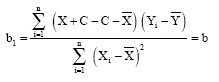 | (4) |
Using Eq. 3:
| (5) |
ESTIMATES OF THE MODEL PARAMETERS WHEN A CONSTANT IS ADDED TO THE DEPENDENT VARIABLE
Suppose d is a constant and we wish to regress H = Y+d on X. Then![]()
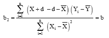 | (6) |
Using Eq. 3:
| (7) |
ESTIMATES OF THE PARAMETERS OF THE MODEL WHEN DIFFERENT CONSTANTS ARE ADDED TO THE DEPENDENT VARIABLE AND INDEPENDENT VARIABLE
Let I = X+e. Then:
Again, If:
Using Eq. 2:
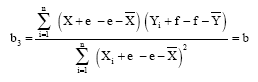 | (8) |
Using Eq. 3:
| (9) |
ESTIMATES OF THE PARAMETERS OF THE MODEL WHEN THE SAME CONSTANT IS ADDED TO THE DEPENDENT AND INDEPENDENT VARIABLES
Given that l is a constant such that M = X+l then:
Again, If:
The estimate of the slope of the regression line is given by:
 | (10) |
The corresponding estimate of the intercept is obtained from Eq. 3 as:
| (11) |
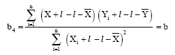
| Table 1: | Regression analysis of the transformed dependent variables on their associated independent variables |
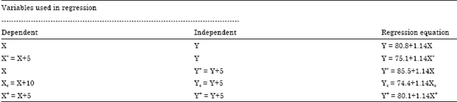 | |
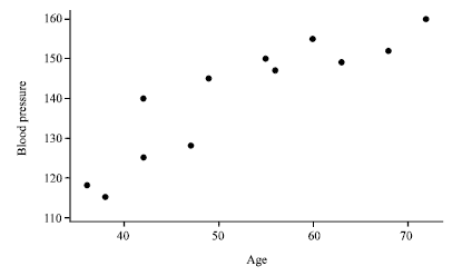 | |
| Fig. 1: | The scatter diagram for determing the nature of the relationship between X and Y |
NUMERICAL ILLUSTRATION
The relationships between the parameter estimates are verified in this section using the data on the age of woman (X) and blood pressure (Y) as given by Spiegel et al. (2000).
To determine nature of the relationship between X and Y, the scatter diagram in Fig. 1 is required.
In Fig. 1, it appears that there is a linear relationship between blood pressure and age of woman. Summary of regression analysis of the various functions of the dependent variable on their corresponding independent variables is given in Table 1.
As we can see from Table 1, the addition of constants to one or both variables involved in regression does not affect the estimate of the slope (β) of the regression line. Moreover, the estimate of the intercept (α) of the regression line involving the transformed values of X and Y is a function of the added constants. These are all in line with results obtained in Eq. 5, 7, 9 and 11.
CONCLUSION
In this study, the influence of transforming variables involved in a simple linear regression model by addition of constants is examined. It has been shown that whether constants are added to one or both variables, the estimate of the slope is not affected. Meanwhile, the estimate of the intercept depends on what constants that have been added. Since the estimated regression equation is a function of the estimates of the slope and intercept, the predictive ability of a regression model is therefore affected by constant addition.
REFERENCES
- Ding, C.S., 2006. Using regression mixture analysis in educational research, practical assessment. Res. Eval., 11: 1-11.
Direct Link - El-Shehawy, S.A., 2008. Selection of a NLR-model by Re-sampling technique. Asian J. Math. Stat., 1: 109-117.
CrossRefDirect Link - Igwenagu, C.M., 2011. Principal component analysis of global warming with respect to CO2 emission in Nigeria: An exploratory study. Asian J. Math. Stat., 4: 71-80.
CrossRefDirect Link - Abd El-Salam, M.E.F., 2011. An efficient estimation procedure for determining ridge regression parameter. Asian J. Math. Stat., 4: 90-97.
CrossRefDirect Link - Abdullah, L. and H. Asngari, 2011. Factor analysis evidence in describing consumer preferences for a soft drink product in Malaysia. J. Applied Sci., 11: 139-144.
CrossRefDirect Link - Olaomi, J.O. and A. Ifederu, 2008. Understanding estimators of linear regression model with AR(1) error which are correlated with exponential regressor. Asian J. Math. Stat., 1: 14-23.
CrossRefDirect Link - Rajarathinam, A. and R.S. Parmar, 2011. Application of parametric and nonparametric regression models for area, production and productivity trends of castor (Ricinus communis L.) crop. Asian J. Applied Sci., 4: 42-52.
CrossRefDirect Link - Steel, R.G.D. and J.H. Torrie, 1981. Principles and Procedures of Statistics: A Biometrical Approach. 2nd Edn., McGraw-Hill, New York, Pages: 633.
Direct Link