
Riccardo Cesari
Universita di Bologna, Dip. MatemateS, viale Filopanti, 5, 40126 Bologna, Italy
Carlo D`Adda
Universita di Bologna, Dip. Scienze Economiche, Strada Maggiore, 45, 40125 Bologna, Italy
Asian Journal of Mathematics & Statistics
Year: 2010 | Volume: 3 | Issue: 2 | Page No.: 52-68


ABSTRACT
During the last 50 years, a considerable effort has been devoted to connecting the expected utility approach to a utility function directly expressed in terms of moments of the probability distribution of an uncertain prospect. We follow the alternative route of providing, for the first time, the theoretical, autonomous foundation of an ordinal utility function of moments, representing rational choices under uncertainty, free of any independence axiom and compatible with many paradoxes of choice and behavior, well documented in the literature.
PDF Abstract XML References Citation
How to cite this article
Riccardo Cesari and Carlo D`Adda, 2010. An Ordinal Utility of Moments for Decisions under Uncertainty. Asian Journal of Mathematics & Statistics, 3: 52-68.
DOI: 10.3923/ajms.2010.52.68
URL: https://scialert.net/abstract/?doi=ajms.2010.52.68
DOI: 10.3923/ajms.2010.52.68
URL: https://scialert.net/abstract/?doi=ajms.2010.52.68
INTRODUCTION
Tobin (1958), in setting, 50 years ago, the microeconomic foundations of the keynesian liquidity preference theory in the light of the Markowitz (1952, 1959) portfolio approach, has shown an important equivalence between the Von Neumann and Morgenstern (1944) expected utility (VNM) and a preference function in mean and standard deviation.
His extension of this result to all two-parameter distributions was subsequently proved incorrect by Samuelson (1967), Borch (1969) and Feldstein (1969) so that a mean-variance analysis has been justified for a long time only under the restrictive assumption of quadratic VNM utility or Gaussian distribution.
Two research areas have therefore attracted considerable interest: one focused on suitable distributional assumptions and one devoted to the most appealing form of the utility function.
Regarding the former, the admissible distributions have been identified by the elliptical class (Chamberlain, 1983; Owen and Rabinowitch, 1983), which is closed under linear transformations of random variables. Elliptical distributions are also known as scale-location parameter distributions (as in Tobin’s conjecture) or linear distributions (Sinn, 1983; Meyer, 1987; Levy, 1989). They include the symmetric stable distributions analyzed by Fama (1971).
In addition, a large amount of work has been done to justify mean-variance (EV) analysis just as a second-order approximation of the expected utility model, avoiding the absurd assumption of quadratic utility (Hicks, 1962; Pratt, 1964; Arrow, 1965) and its property of increasing risk aversion and decreasing asset demand as wealth increases, making risky assets inferior goods.
Early studies concerning EV as an approximation of expected utility were carried out by Samuelson (1967, 1970), Tsiang (1972, 1974) and Rubinstein (1973), also including higher-order moments in a generalized approach.
Levy and Markowitz (1979), Kroll et al. (1984), Reid and Tew (1986) and Markowitz (1987) assess the effectiveness of the EV approximation, confirming Markowitz’s intuition that mean-variance is, in practice, as efficient as expected utility in selecting optimal portfolios.
Even in more theoretical works, such as Hakansson (1972), Baron (1977) and Bigelow (1993), the aim was to investigate the consistency between mean-variance (or moment-) utility and the VNM axioms or utility function, providing restrictions to a simultaneous validity of both approaches.
However, any attempt to make expected utility and moment utility equivalent does not seem a truly compelling task.
Many authors (Borch, 1969, 1973; Levy, 1989) are, in fact, well aware of the different set-up of the two approaches, particularly when the arguments of moment utility are not confined to mean and variance but include all relevant moments of the probability distributions.
Moreover, during the last century, a number of works, from Knight (1921) to Keynes (1921), from Hicks (1935, 1962) to Marschak (1938), from Lange (1944) to Simpson (1950), expressed intriguing suggestions on variance, dispersion and higher-order moments as relevant parameters directly influencing the agent’s decisions under uncertainty.
In this study, we develop the foundations of an ordinal utility of moments as a rational and autonomous criterion of choice under uncertainty, showing that it dissolves all the best known behavioral paradoxes which are still embarrassing the expected utility theory. This ordinal approach is strongly reminiscent of standard microeconomic theory and it could be used to reset and generalize both assets demand theory and asset pricing models.
FOUNDATIONS
It is well known that the theory of choice under uncertainty assumes that preferences are defined over the set of probability distribution functions (Savage, 1954; DeGroot, 1970).
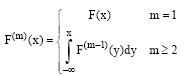
Confining ourselves, for ease of exposition, to the case of univariate distributions, we assume that the essential information concerning any distribution F is contained in the m-dimensional vector of moments M ≡ (μ, μ(2), μ(3),...., μ(m)) where, μ is the mean and μ(s) is the s-order central moment in original units, so that (μ(s))s is the usual central moment of order s≥2.
Note that, instead of central moments, noncentral moments could, equivalently, be used. Moreover, scale, location and dispersion parameters can be considered in the case of distributions (e.g., stable) for which moments do not exist.
The existence of an ordinal utility of moments is obtained under the assumption of a preference order satisfying the axioms of (1) asymmetry, (2) transitivity and (3) continuity (Appendix).
Assumption of Preference Order
Let Q⊆Rm be a rectangular subset of Rm (the cartesian product of m real intervals), whose elements are the m-dimensional vectors of moments, M∈Q. Let › be a preference order i.e., a binary relation defined by a subset ![]() of the Cartesian product QxQ, whose elements are the ordered pairs of vectors (Ma, Mb).
of the Cartesian product QxQ, whose elements are the ordered pairs of vectors (Ma, Mb).
We write Ma›Mb instead of (Ma,Mb)![]() and we say that Ma is preferred to Mb, corresponding to Fa is preferred to Fb for distribution functions.
and we say that Ma is preferred to Mb, corresponding to Fa is preferred to Fb for distribution functions.
Clearly, or Ma›Mb or Ma![]() Mb and both cannot hold: in fact, or (Ma, Mb)
Mb and both cannot hold: in fact, or (Ma, Mb) ![]() or (Ma, Mb)
or (Ma, Mb) ![]() .
.
We write Ma~Mb (equivalence) if and only if Ma![]() Mb and Mb
Mb and Mb![]() Ma.
Ma.
Theorem 1: Of Complete Preferences
The preference order is complete.
Theorem 2: Of Negatively Transitive Preferences
The preference order is negatively transitive.
Theorem 3: Of Equivalence Classes
The equivalence ~ is reflexive, symmetric and transitive.
Theorem 4: Of Ordinal Utility on Moments
Under Axioms I, II, III there is a real function H: Q→R which represents the preferences ›, i.e., such that, for every Ma, Mb∈Q:
| (1) |
The function H is unique up to any order-preserving transformation Ø:
| (2) |
The function H is called an ordinal utility because it just represents the given preference order › in terms of otherwise arbitrary real numbers (utils).
Theorem 5: Of Continuous Utility
Under Axioms I, II, III and the usual relative topology for Q (intersection of Q with the set of all open rectangles in Rm, including arbitrary unions and finite intersections; Debreu (1959), Rader (1963)), the utility function H is continuous if and only if, for every Ma∈Q, the sets {Mb∈Q: Ma›Mb} and {Mb∈Q: Mb›Ma} belong to the topology.
In the following, we assume that H is continuous with bounded first order partial derivatives. The usual concepts available in the theory of choice under uncertainty can be extended to our approach.
Let F, G be two probability distributions with relevant moment vectors:
MF ≡ (μF, μF(2), μF(3),...., μF(m) ) and MG≡(μG, μG(2), μG(3),...., μG(m)), respectively. Let H(M) be a differentiable utility function.
Definition of Non Satiation
The utility H is non satiated if, for every δ>0:
| (3) |
In differential terms: ![]() .
.
Definition of Risk Aversion
A utility H is risk averse if, for every F:
| (4) |
Note that for m = 2, risk aversion means ![]() ; for m≥3, a negative marginal utility of volatility
; for m≥3, a negative marginal utility of volatility ![]() does not imply risk aversion.
does not imply risk aversion.
Definition of Certainty Equivalent
The certainty equivalent of F is defined as the amount CF such that:
| (5) |
Definition of Risk
Given two distributions F, G with equal mean, μF = μG, we say that F is less risky than G if H(MF)> H(MG) for every risk averse utility H.
Definition of Stochastic Dominance
Given two distribution functions, F, G defined over the same support, we have mth-order stochastic dominance of F over G, F›mG, m≥1, if F≠G and:
where:
 |
Clearly, if F›mG then F›m+1G.
We recall a well known result linking stochastic dominance and VNM expected utility functions.
Theorem 6 on Stochastic Dominance and Expected Utility
We have:
| • | F›1G ⇔ EF (U(x))≥EG(U(x)) for every U with U’≥0 |
| • | F›2G ⇔ EF (U(x))≥EG(U(x)) for every U with U’≥0, U”≤0 |
| • | F›3G ⇔ EF (U(x))≥EG(U(x)) for every U with U’≥0, U”≤0, U”’≥0 |
Therefore, first order stochastic dominance means increasing VNM utilities; second order stochastic dominance means increasing and concave VNM utilities.
This is no longer true for the moment ordinal utility.
Theorem 7 on Stochastic Dominance and Moment Utility
If F›mG then MF ≡ (μF, μF(2), μF(3),...., μF(m))≠(μG, μG(2), μG(3),...., μG(m)) ≡ MG and (-1)k-1μF(k)> (-1)k-1μG(k) for the smallest k for which μF(k)≠μG(k).
As special cases we have:
| • | If F›1G then μF>μG |
| • | If F›2G then (μF>μG) or (μF = μG and μF(2)<μG(2)) |
| • | If F›3G then (μF>μG) or (μF = μG and μF(2)<μG(2)) or (μF = μG and μF(2) = μG(2) and μF(3)>μG(3)) |
In the first case, in particular, it does not necessarily follow (even if it is, however, plausible) that H(MF)>H(MG) whenever higher order moments are relevant. In particular, Allais (1953, 1979) assumes that F›1G implies H(F)>H(G) (axiom of absolute preference). In the expected utility approach it is equivalent to assume U’>0 (nonsatiation).
INDIFFERENCE PRICING AND THE (DIS)SOLUTION OF PARADOXES
The Von Neumann-Morgenstern (1944) theory of choice under uncertainty has long been the standard approach to model the maximizing behavior of agents in financial markets. The basic result is the existence of a utility function U(.) (the VNM utility) describing the optimal decisions of an investor as those maximizing the expected utility of his or her future wealth E(U( ![]() )). This beautiful result was obtained at the cost of a special and controversial axiom concerning the structure of preferences in the case of uncertainty, the so-called independence axiom, inducing a linear dependence between utility and probabilities.
)). This beautiful result was obtained at the cost of a special and controversial axiom concerning the structure of preferences in the case of uncertainty, the so-called independence axiom, inducing a linear dependence between utility and probabilities.
In fact, the independent axiom assumes that randomization is irrelevant: it says that if A›B then pA+(1-p)C›pB+(1-p)C (Machina, 1987; Fishburn, 1982, 1988 and the seminal work in Von Neumann and Morgenstern, 1944, especially chapter 1 and Appendix, where, considering their penetrating results, they ask themselves, p.28, Have we not shown too much?).
The approach followed above replaces the VNM expected utility with the more fundamental and less demanding ordinal utility H(E( ![]() ), Std (
), Std ( ![]() ),...), allowing us to avoid the main flaws of the former and providing us with a generalized framework for optimal behavior in both complete and incomplete markets. In particular, note that H is a utility of expectations and not an expectation of utilities.
),...), allowing us to avoid the main flaws of the former and providing us with a generalized framework for optimal behavior in both complete and incomplete markets. In particular, note that H is a utility of expectations and not an expectation of utilities.
Note also that this approach is different from (and much simpler than) other generalizations (non-expected utility approaches) suggested in the literature after Allais (1953) contribution to the empirical critique of the VNM expected utility theory.
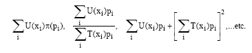
In fact, in most cases, including Allais (1979), Kahneman and Tversky (1979), Chew (1983), Fishburn (1983), Machina (1982) and many others, the utility function is a function of moments of a Bernoullian utility U, or a nonlinear function of both Bernoullian utilities and subjective probabilities:
 |
In our case, we obtain a more general result based on more intuitive elements:
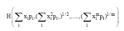 | (6) |
Moreover, it is well known that the expected utility can be approximated by a particular function of m central moments:
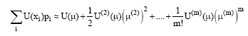 | (7) |
where, U(j) is the j-th derivative of U, but this is only a special (polynomial) case of H and is not always able to account for the observed phenomena.
The utility of moments is perfectly compatible with the empirical observations in all well known behavioral paradoxes, described in terms of games and lotteries.
In order to show this compatibility we use the so called utility-indifference pricing (Henderson and Hobson, 2009), which can be applied in all cases of personal valuation of non-traded assets and incomplete markets.
For the sake of simplicity, let us consider the two-moment ordinal utility.
Let W be the current wealth of the decision maker and ![]() be the random variable representing the game, with mean MG and vol ΣG. Future wealth, in case of a decision to gamble, is given by:
be the random variable representing the game, with mean MG and vol ΣG. Future wealth, in case of a decision to gamble, is given by:
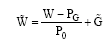 | (8) |
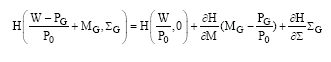
where, W-PG is wealth left after payment for the game, invested at the riskless rate r = 1/P0-1 (often set to zero) and the personal indifference price PG is defined as the price at which the agent is indifferent to paying the price and entering the game or paying nothing and avoiding the game:
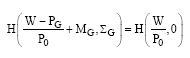 | (9) |
In the l.h.s., using a Taylor series approximation for small risks (Pratt, 1964), we have:
 | (10) |
so that, imposing Eq. 9 and simplifying, we obtain:
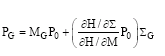 | (11) |
where, the term in brackets is the (negative) personal price of the vol, Pσ and it is independent of monotonic transformation of H. Therefore, the indifference price, PG, of the game is obtained as moment quantities, MG, ΣG, times subjective moment prices, P0, Pσ.
Moreover, Eq. 11 can be easily generalized to higher moments (skewness Γ and kurtosis Ψ):
| (12) |
and this version will be used in the following to show that the behavior of a moment-utility maximizer is perfectly compatible with all the proposed paradoxes, from St. Petersburg (1713) to Friedman and Savage (1948), Allais (1953, 1979) and Kahneman and Tversky (1979).
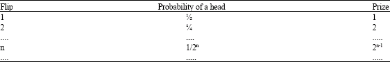
| Table 1: | The St. Petersburg game |
 | |
The St. Petersburg Paradox
The name of the paradox is due to the solution, proposed by Daniel Bernoulli in 1738 to a question posed by his cousin Nicolas Bernoulli, in a letter dated September 9th, 1713. Note that at that time, the method to value an uncertain prospect was established by Christian Huygens in 1657 as the mathematical expectation of the gain (Hacking, 1975). Peter tosses a coin and continues to do so until it should land heads when it comes to the ground. He agrees to give Paul one ducat if he gets heads on the very first throw, two ducats if he gets it on the second, four if on the third, eight if on the fourth and so on, so that with each additional throw, the number of ducats he must pay is doubled.
Paul is the player: if he obtains heads at the first flip he wins 1, at the second flip he wins 2,..., at the n-th flip he wins 2n-1 and so on. The question is to determine a fair price, P(G), to enter the game.
Clearly, the price must be at least 1 (the minimum gain), but the expected gain is infinite (Table 1).
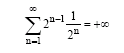 |
However, as Nicolas Bernoulli observed in stating the paradox, nobody would pay an arbitrarily large amount to play the game: it has, he said, to be admitted that any fairly reasonable man would sell his chance, with great pleasure, for twenty ducats.
The famous Bernoulli solution, in log terms, provided a path-breaking device, introducing the concept of utility (moral expectation) and reducing expectation to a finite value:
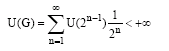 |
Alternatively, the price, P(G), of the game can be obtained, in our approach, by considering the sequential game as a one-shot game (a lottery) with an infinity of tickets, identified by natural numbers (1, 2,..., n,.....) with decreasing probability of extraction (½, ¼,...,½n,....) and increasing rewards (1, 2,..., 2n-1,...). This means that the original game is a portfolio of sub-games Gn n≥1 or Arrow-Debreu securities (one for each row in the table above), the n-th of which implies a prize of 2n-1 if we get heads at the n-th flip and zero otherwise.
Clearly, each ticket could be sold separately at its price P(Gn) and the price of the lottery is the sum of the prices of all tickets.
We show that a two-moment utility approach is sufficient to solve the paradox.
| Table 2: | The first two moments of the St. Petersburg game |
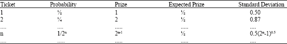 | |
For each ticket n, the expected value is always ½ and the standard deviation is 0.5 (2n-1)0.5:
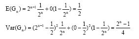 |
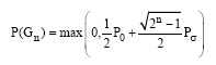
Considering the first two moments (Table 2) the price of the n-th ticket is, from Eq. 12:
 |
where, the limited liability provision has been applied and the price of the game is simply the sum of the (non negative) prices of all tickets:
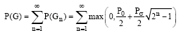 |
For example, if P0 = 1 and Pσ = -0.134 then P(Gn) = 0 for n>5 and P(G) = 1.507. Coin tosses beyond the fifth have no economic value. Note that in this game-situation, Pσ is not a proper market price but just the gambler’s personal price of volatility. Analogously for higher-order moments; a refined price P(G) could also be obtained using higher moments: the skewness of the n-th ticket is [0.25 (2n-1) (2n-1-1)]1/3; the kurtosis is [(2n-1) ((2n-1)3+1)/2n+4]1/4.
The Friedman and Savage (1948) Paradox
In their classical article, Friedman and Savage (1948) observed the difficulty of combining the belief in diminishing marginal utility and the observation that the same individual buy insurance as well as lottery tickets. Clearly, the first choice is evidence of risk aversion but the second one can be rationalized only by a risk loving behavior, being well known that lotteries are largely unfair games, accepted only by individuals having a strong preference for risk.
The clever solution they proposed, in the framework of the Von Neumann-Morgenstern theory, just published a few years before, was based on a complex hypothesis concerning the shape of the utility function, made by three segments, concave-convex-concave, where current income is in the initial convex segment (ivi, paragraph IV).
In terms of moment utility the solution is much simpler and it clarify that skewness is the key element behind the observed behavior.
A typical lottery represents a large chance of losing a small amount (the price of the lottery ticket) plus a small change of winning a large amount (a prize).
Viceversa, the game against which you buy insurance, paying the premium π, contains a small chance of a much larger loss and a large chance of no loss. Let L and J be, respectively, the two random variables so that L (lottery) is preferred to 0 as well as -π is preferred to J:
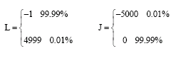 |
| Table 3: | The first three moments of the Friedman-Savage lottery (L) and insurance (J) |
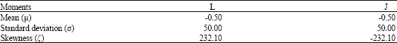 | |
Let us calculate the first three moments of L and J (Table 3).
Mean and standard deviation are the same but skewness is reversed in sign, with L having a large, positive skewness and J a large, negative one. Assuming the following prices of the three moments: P0 = 1, Pσ = -0.34, Pζ = 0.1 we obtain the prices P(L) = 5.71>0 and P(J) = -40.70<0 so that the ticket is bought with pleasure (and considered cheap) and up to 40.7 money units could be willingly paid to avoid the insurable risk.
The Allais Paradox
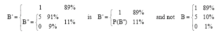
The Allais (1953) paradox was the first factual evidence against expected utility. In fact, asking people to choose between games A and B, where A gives 1 million with certainty and B gives 1 million with 89% probability and 0 or 5 millions with, respectively, 1 and 10% probabilities:
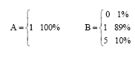 |
people prefer in large majority A to B: A›B.
Then, asking them to choose between A’ and B’ defined by:
 |
the same people very often prefer B’ to A’: B’›A’.
The paradox stems from the fact that, from A›B, the expected utility approach deduces A’›B’, which is at variance with the experimental evidence (Allais reports 53% of cases of violation of the logical implication).
In fact, A›B means:
but collecting U(1) and adding to both members of the inequality 0.89U(0) you obtain, algebraically:
i.e., A’›B’, against the empirical evidence.
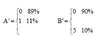
| Table 4: | The first four moments of the Allais games |
 | |
According to Allais, either people in experimental situations do not use the rational thinking used in real world decision-making, or people do not follow the expected utility paradigm.
In fact, using our approach, the rationality of the actual choices may be easily recognized.
Considering each lottery as an asset, the first four moments are in Table 4.
Assuming the following prices of the four moments: P0 = 1, Pσ = -0.34, Pζ = 0.01, Pκ = -0.001 we obtain the prices of the lotteries: P(A) = 1>P(B) = 0.994 and P(A’) = 0.007< P(B’) = 0.008, in accordance with the Allais experiments.
This means that, using the Marschak triangle as in Machina (1987), the indifference curves in our approach are nonlinear in the probabilities and may display a ‘fanning out’ effect from the sure event A, as implied by actual behavior.
The Kahneman and Tversky (1979) Paradox
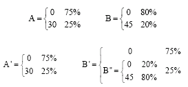
In a famous experiment, a systematic violation of the independence axiom was documented: 80% of 95 respondents preferred A to B where:
65% preferred B’ to A’ where:
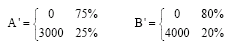 |
and more than 50% of respondents violated the independent axiom, given that, if Q pays 0 for sure, then:
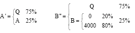 |
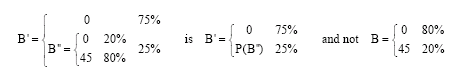
and B” is considered equal to B’ in terms of outcomes and probabilities.
Note that treating lotteries as assets implies that linear combinations such as 0.75Q+0.25A are meaningful and P(0.75Q+0.25A) = 0.25P(A)≠P(A’).
The point is that, in terms of valuation, B’ and B” are not the same asset and B” is equivalent to:
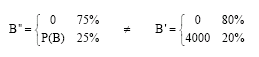 |
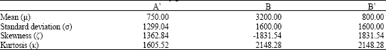
| Table 5: | The fist four moments of Kahneman-Tversky games |
 | |
| Table 6: | The first four moments of the Tversky-Kahneman games |
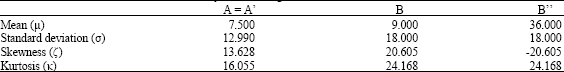 | |
Using the first four moments in Table 5 and assuming the following prices of the four moments: P0 = 1, Pσ = -0.2, Pζ = 0.1, Pκ = -0.001 we obtain the prices of the lotteries: P(A) = 3000>P(B) = 2694.70 and P(A’) = 624.87<P(B’) = 661.01, in accordance with the experimental results. Note also that P(B”) = 561.28<P(A’)<P(B’).
The Tversky and Kahneman (1981) Paradox
Most subjects, confronted with the following alternatives: A versus B and A’ versus B’, prefer B to A but also A’ to B’ where:
 |
The paradox (reversal or isolation effect) stems from the fact that not only A = A’ but also B = B’ in terms of ultimate outcomes and probabilities.
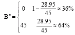
However, from the point of view of our theory of valuation and choice, the two-stage frame in B’ is not irrelevant: in B, not 0 means 45; in B’, not 0 means a new game B”, which can be sold for a certain price.
Using the first four moments in Table 6 and assuming the following prices of the four moments: P0 = 1, Pσ = -0.2, Pζ = 0.05, Pκ = -0.1, we obtain the prices of the lotteries: P(A) = 3.98 <P(B) = 4.01 and P(A’) = 3.98>P(B’) = 3.84, being 30>P(B”) = 28.95. This result is in accordance with the Tversky and Kahneman (1981) experiment, showing that, in effect, no paradox is implied in the observed behavior.
In particular, note, once again, that in terms of valuation:
 |
and the risk-neutral probabilities for B”, for which the personal price of B” is the expected value:
are given by:
 |
This observation also holds for the Markowitz (1959) formulation of Allais’s experiment:
 |
CONCLUSIONS
After Tobin (1958), considerable effort has been devoted to connecting the expected utility approach to a utility function directly expressed in terms of moments. In contrast with this approach, we have provided the theoretical foundation of an ordinal utility function of moments which is free of any independence axiom and compatible with all the behavioral paradoxes documented in recent and less recent works on decisions under uncertainty. This moment-utility can be used as the starting point for a new formulation of asset demand models and asset pricing, having more general properties and greater flexibility than existing expected utility results. Future research could be addressed in this promising direction.
APPENDIX: BASIC AXIOMS AND PROOFS OF THE THEOREMS
Let (Ω, ![]() ,
, ![]() ) be a standard probability space, Ω being the set of elementary events (states of the world),
) be a standard probability space, Ω being the set of elementary events (states of the world), ![]() the set (σ-algebra) of subsets of Ω (events),
the set (σ-algebra) of subsets of Ω (events), ![]() a (subjective) probability measure of the events. Given the set A of all possible actions or decisions, all couples (ω,a) with ω∈Ω and a∈A, are mapped onto a real vector of monetary consequences c∈Rn, the Euclidean space of n-dimensional real vectors, so that X (ω,a) = c or Xa (ω) = c is a random variable and Fa∈F is its probability distribution function. Clearly, the preferences over acts in A are, equivalently, preferences over the set of random variables Xa as well as preferences over the set F of distribution functions. Let us confine ourselves, for ease of exposition, to the case of univariate distributions (n = 1) and assume that the essential information concerning any distribution F is contained in the m-dimensional vector of moments M≡(μ, μ(2), μ(3),...., μ(m)) where μ is the mean and μ(s) is the s-order central moment in original units:
a (subjective) probability measure of the events. Given the set A of all possible actions or decisions, all couples (ω,a) with ω∈Ω and a∈A, are mapped onto a real vector of monetary consequences c∈Rn, the Euclidean space of n-dimensional real vectors, so that X (ω,a) = c or Xa (ω) = c is a random variable and Fa∈F is its probability distribution function. Clearly, the preferences over acts in A are, equivalently, preferences over the set of random variables Xa as well as preferences over the set F of distribution functions. Let us confine ourselves, for ease of exposition, to the case of univariate distributions (n = 1) and assume that the essential information concerning any distribution F is contained in the m-dimensional vector of moments M≡(μ, μ(2), μ(3),...., μ(m)) where μ is the mean and μ(s) is the s-order central moment in original units:
Definition of s-order modified central moment: 
Note that (μ(s))s is the usual central moment of order s≥2.
Let Q⊆Rm be a rectangular subset of Rm (the Cartesian product of m real intervals), whose elements are the m-dimensional vectors of moments, M∈Q.
Assumption of Preference Order
Let › be a preference order i.e., a binary relation defined by a subset ![]() of the Cartesian product QxQ, whose elements are the ordered pairs of vectors (Ma,Mb).
of the Cartesian product QxQ, whose elements are the ordered pairs of vectors (Ma,Mb).
We write Ma›Mb instead of (Ma,Mb) ![]() and we say that Ma is preferred to Mb, corresponding to Fa is preferred to Fb.
and we say that Ma is preferred to Mb, corresponding to Fa is preferred to Fb.
Clearly, or Ma›Mb or Ma![]() Mb and both cannot hold: in fact, or (Ma,Mb)
Mb and both cannot hold: in fact, or (Ma,Mb) ![]() or (Ma,Mb)
or (Ma,Mb) ![]() .
.
I. Axiom of Asymmetric Preferences
We assume that › is asymmetric i.e., that:
| (A.2) |
The relation is therefore irreflexive and, moreover, if Mb![]() Ma then two alternative cases are possible: either Ma›Mb or Ma
Ma then two alternative cases are possible: either Ma›Mb or Ma![]() Mb.
Mb.
In the latter case we say that Ma and Mb are equivalent and we write Ma ~ Mb.
Definition of Equivalence
Ma ~ Mb if and only if Ma![]() Mb and Mb
Mb and Mb![]() Ma
Ma
Theorem 1 of Complete Preferences
Given Ma, Mb ∈Q then one and only one case holds: Ma›Mb or Mb›Ma or Ma~Mb.
Proof: It is easy to show that any two cases are a contradiction. ![]()
II. Axiom of Transitive Preferences
We assume that › is transitive:
| (A.3) |
Definition of Weak Order
The preference order › is a weak order if it is asymmetric and transitive.
Definition of Negatively Transitive Preferences
If Ma![]() Mb and Mb
Mb and Mb![]() Mc then Ma
Mc then Ma![]() Mc.
Mc.
Lemma 1
› is negatively transitive if and only if, for every Ma, Mb, Mc∈Q, Ma›Mb implies Ma›Mc or Mc›Mb.
Proof: Under negative transitivity, if Ma›Mb but Ma![]() Mc and Mc
Mc and Mc![]() Mb then by negative transitivity Ma
Mb then by negative transitivity Ma![]() Mb against the assumption.
Mb against the assumption.
Viceversa, if Ma›Mb implies Ma›Mc or Mc›Mb and negative transitivity is false we have from Ma![]() Mc and Mc
Mc and Mc![]() Mb that Ma›Mb so that Ma›Mc or Mc›Mb, in both cases a contradiction.
Mb that Ma›Mb so that Ma›Mc or Mc›Mb, in both cases a contradiction. ![]()
Theorem 2 of Negatively Transitive Preferences
Asymmetric and transitive preferences are equivalent to asymmetric and negatively transitive.
Proof: Under transitivity if Ma›Mb and Mb›Mc then Ma›Mc; therefore, by asymmetry, if Mb![]() Ma and Mc
Ma and Mc![]() Mb then Mc
Mb then Mc![]() Ma which is negative transitivity.
Ma which is negative transitivity.
Viceversa, under negative transitivity, if Ma›Mb and Mb›Mc then, from Lemma 1, (Ma›Mc or Mc›Mb) and (Mb›Ma or Ma›Mc). But, by asymmetry, Mb![]() Ma and Mc
Ma and Mc![]() Mb so that Mc›Mb and Mb›Ma are false. Therefore Ma›Mc which means transitivity.
Mb so that Mc›Mb and Mb›Ma are false. Therefore Ma›Mc which means transitivity. ![]()
Theorem 3 of Equivalence Classes
The equivalence ~ is reflexive, symmetric and transitive and we have:
| (A.4) |
Moreover, › on Q|~ (the set of equivalence classes of Q under ~) is a strict order i.e., it is a weak order and for every equivalence class MA, MB ∈Q|~ one and only one case holds: MA›MB or MB›MA (weak connectedness).
Proof: The equivalence is clearly reflexive and symmetric. Suppose it is not transitive: Ma~Mb and Mb~Mc but Ma ~ Mc is false. Then, by definition, either Ma›Mc or Mc›Ma. From Lemma 1, in the first case, Ma›Mb or Mb›Mc; in the second case Mc›Mb or Mb›Ma, in contradiction with the hypothesis.
If Ma›Mb and Ma~Mc then by Theorem 1 and Lemma 1 we have Mc›Mb. If Ma›Mb and Mb~Mc then by Theorem 1 and Lemma 1 we have Ma›Mc.
Finally, › on Q|~ is a weak order, being asymmetric and negative transitive: under symmetry, if MA›MB and MB›MA then exist Ma, Ma’ in MA and Mb, Mb’ in MB such that Ma~Ma’, Mb~Mb’ and Ma›Mb and Mb’›Ma’. From (A.4) Ma›Mb’ and Mb’›Ma which is a contradiction; for negative transitivity, if MA›MB then Ma›Mb for any Ma in MA and Mb in MB and if Mc is any vector in MC then we have, from Lemma 1, Mc›Mb or Ma›Mc. Therefore, MC›MB or MA›MC.
For weak connectedness, given that MA and MB are disjoint, from Theorem 1, either Ma›Mb or Mb›Ma for every Ma in MA and Mb in MB. Therefore, either MA›MB or MB›MA. ![]()
III. Axiom of Continuity
There is a countable subset D⊆Q|~ that is›-dense in Q|~ i.e., for every MA, MC ∈Q|~\D, MA›MC there is MB∈D such that:
| (A.5) |
Note that the subset of rational numbers is >-dense and <-dense in the set of real numbers.
Theorem 4 of Ordinal Utility on Moments
Proof: The proof follows the steps as in Fishburn (1970).![]()
Theorem 5 of Continuous Utility
Proof: See Debreu (1964).![]()
Theorem 6 on Stochastic Dominance and Expected Utility
Proof: (i) using integration by parts:
Therefore, if F(x)≤G(x) then EF(U(x))≥EG(U(x)). Viceversa, if EF(U(x))≥EG(U(x)) let I be an interval in which F(x)>G(x) and let χI be the indicator function of I. Define:
so that U’(x)≡χI(x)≥0 and inserted into the above equation gives a contradiction. For (ii) and (iii) Fishburn and Vickson (1978) and Whitmore (1970).![]()
Theorem 7 on Stochastic Dominance and Moment Utility
Proof: Apply Fishburn (1980, theorem 1) and the relation between central, μ and non central, v, moments:
 |
REFERENCES
- Allais, M., 1953. Le comportement de l'homme rationnel devant le risque: Critique des postulats et axiomes de l'ecole americaine. Econometrica, 21: 503-546.
Direct Link - Baron, D.P., 1977. On the utility theoretic foundations of mean-variance analysis. J. Finance, 32: 1683-1697.
Direct Link - Bigelow, J.P., 1993. Consistency of mean-variance analysis and expected utility analysis: A complete characterization. Econ. Lett., 43: 187-192.
Direct Link - Borch, K., 1969. A note on uncertainty and indifference curves. Rev. Econ. Stud., 36: 1-4.
Direct Link - Borch, K., 1973. Uncertainty and indifference curves: A correction. Rev. Econ. Stud., 40: 141-141.
Direct Link - Chamberlain, G., 1983. A characterization of the distributions that imply mean-variance utility functions. J. Econ. Theory, 29: 185-201.
Direct Link - Chew, S.H., 1983. A generalization of the quasilinear mean with applications to the measurement of income inequality and decision theory resolving the Allais paradox. Econometrica, 51: 1065-1092.
Direct Link - Debreu, G., 1964. Continuity properties of Paretian utility. Int. Econ. Rev., 5: 285-293.
Direct Link - Feldstein, M.S., 1969. Mean-variance analysis in the theory of liquidity preference and portfolio selection. Rev. Econ. Stud., 36: 5-12.
Direct Link - Fishburn, P.C., 1980. Stochastic dominance and moments of distributions. Math. Operat. Res., 5: 94-100.
Direct Link - Friedman, M. and L.J. Savage, 1948. The utility analysis of choices involving risk. J. Polit. Econ., 56: 279-304.
Direct Link - Hakansson, N.H., 1972. Mean-variance analysis in a finite world. J. Financ. Quant. Anal., 7: 1873-1880.
Direct Link - Kahneman, D. and A. Tversky, 1979. Prospect theory: An analysis of decision under risk. Econometrica, 47: 263-292.
CrossRefDirect Link - Kroll, Y., H. Levy and H.M. Markowitz, 1984. Mean-variance versus direct utility maximization. J. Finance, 39: 47-61.
Direct Link - Levy, H., 1989. Two-moment decision models and expected utility maximization: Comment. Am. Econ. Rev., 79: 597-600.
Direct Link - Levy, H. and H.M. Markowitz, 1979. Approximating expected utility by a function of mean and variance. Am. Econ. Rev., 69: 308-317.
Direct Link - Machina, M.J., 1982. Expected utility` analysis without the independence axiom. Econometrica, 50: 277-323.
Direct Link - Machina, M.J., 1987. Choice under uncertainty: Problems solved and unsolved. Econ. Perspect., 1: 121-154.
Direct Link - Meyer, J., 1987. Two-moment decision models and expected utility maximization. Am. Econ. Rev., 77: 421-430.
Direct Link - Owen, J. and R. Rabinovitch, 1983. On the class of elliptical distributions and their applications to the theory of portfolio choice. J. Finance, 38: 745-752.
Direct Link - Rader, T., 1963. The existence of a utility function to represent preferences. Rev. Econ. Stud., 30: 229-232.
Direct Link - Reid, D.W. and B.V. Tew, 1986. Mean-variance versus direct utility maximization: A comment. J. Finance, 41: 1177-1179.
Direct Link - Rubinstein, M., 1973. The fundamental theorem of parameter-preference security valuation. J. Fin. Quant. Anal., 1: 61-69.
Direct Link - Samuelson, P.A., 1967. General proof that diversification pays. J. Financ. Quant. Anal., 2: 1-13.
Direct Link - Samuelson, P.A., 1970. The fundamental approximation theorem of portfolio analysis in terms of means, variances and higher moments. Rev. Econ. Stud., 37: 537-542.
Direct Link - Tobin, J., 1958. Liquidity preference as behavior toward risk Rev. Econ. Stud., 25: 65-86.
Direct Link - Tsiang, S.C., 1972. The rationale of the mean-standard deviation analysis, skewness preference and the demand for money. Am. Econ. Rev., 62: 354-371.
Direct Link - Tsiang, SC., 1974. The rationale of the mean-standard deviation analysis: Reply and errata for original article. Am. Econ. Rev., 64: 442-450.
Direct Link - Tversky, A. and D. Kahneman, 1981. The framing of decisions and the psychology of choice. Science, 211: 453-458.
Direct Link - Von Neumann, J. and O. Morgenstern, 1944. Theory of Games and Economic Behavior. 1st Edn., Princeton University Press, Princeton, USA., Pages: 739.
Direct Link