
Karim Solaimani
GIS and RS Centre, University of Agriculture and Natural Resources, P.O. Box 737, Sari, Iran
Asian Journal of Applied Sciences
Year: 2009 | Volume: 2 | Issue: 6 | Page No.: 486-498


ABSTRACT
The present study aims to utilize an Artificial Neural Network (ANN) to modeling the rainfall-runoff relationship in a catchment area located in Iran. The study illustrates the applications of the feed forward back propagation for the rainfall forecasting with various algorithms with performance of multi-layer perceptions. The type of used data in ANN environment was 17 years monthly hydrometric and climatic data. For the operated model 14 years but for the validation/testing of the model 3 years data was applied. The results of this study explored that the capabilities of ANNs and the performance of this tool would be compared to the conventional approaches used for stream flow forecast. The estimated statistical results of the Root Mean Square Error (RMSE) and coefficient of determination (r) measures were calculated foe the used models of 1, 2 and 3 consequently: 2.5, 0.47; 1.57, 0.96; 0.2, 0.998. The results extracted from the comparative study indicated that the Artificial Neural Network method is more appropriate and efficient to predict the river runoff than classical regression model. Efficiency of the used model 1 is facilitated for regular temperature data as input component with using two stations, model 2 for precipitation with using five stations and , model 3 for rainfall, average temperature and flow data as participation with using six stations. It is concluded that model 3 provided more accurate and satisfied results than the other used models.
PDF Abstract XML References Citation
How to cite this article
Karim Solaimani, 2009. A Study of Rainfall Forecasting Models Based on Artificial Neural Network. Asian Journal of Applied Sciences, 2: 486-498.
DOI: 10.3923/ajaps.2009.486.498
URL: https://scialert.net/abstract/?doi=ajaps.2009.486.498
DOI: 10.3923/ajaps.2009.486.498
URL: https://scialert.net/abstract/?doi=ajaps.2009.486.498
INTRODUCTION
Rainfall-runoff models play an important role in water resource management planning; different types of models with various degrees of complexity have been developed for this purpose. These models, regardless to their structural diversity, generally fall into three broad categories; namely, black box or system theoretical models, conceptual models and physically-based models (Singh and Frevert, 2002a, b). Black box models normally contain no physically-based input and output transfer functions and therefore are considered to be purely empirical models. Conceptual rainfall-runoff models usually incorporate interconnected physical elements with simplified forms and each element is used to represent a significant or dominant constituent hydrologic process of the rainfall-runoff transformation Hogue et al. (2006). Conceptual rainfall-runoff models have been widely employed in hydrological modeling. Some of the well-known conceptual models include the Stanford Watershed Model (Crawford and Burges, 2004), Sacramento Soil Moisture Accounting (SAC-SMA) model, (Hsu et al., 1995), Xinanjiang Model (Tan and Connor, 1996; Zhang and Govindaraju, 2003; Zhao, 1992), the Soil Moisture Accounting and Routing (SMAR) Model (Connell et al., 1970; Tan and Connor, 1996) and the Tank Model (Sugawara, 1961, 1995). Conceptual models are reliable in forecasting the most important features of the hydrograph (Kitanidis and Bras, 1980a, b). In comparison with the black box models, conceptual models have potential for evaluating land-use impact on hydrological processes based on relationships of the model parameters to measurable physical characteristics development (Hogue et al., 2006). It seems reasonable to expect that conceptual models would prove to be more faithful in simulating rainfall-runoff process due to it’s physical basis. There has been a tremendous growth in the interest of application the ANNs in rainfall-runoff modeling during 1990s (Dawson and Wilby, 1998; Hsu, et al., 1995; Singh and Frevert, 2002a, b; Sajikumar and Thandaveswara, 1999; Smith and Eli, 1995; Tokar and Johnson, 1999; Tokar and Markus, 2000; Tan and Connor, 1996). Artificial Neural Network were usually assumed to be powerful tools for functional relationship establishment or nonlinear mapping in various applications. Cannon and Whitfield (2002) found ANNs to be superior to linear regression procedures. Shamseldin (1997) examined the effectiveness of rainfall-runoff modeling with ANNs by comparing their results with the Simple Linear Model (SLM), the seasonally based Linear Perturbation Model (LPM) and the Nearest Neighbor Linear Perturbation Model (NNLPM) and concluded that ANNs could provide more accurate discharge forecasts than some of the traditional models. The ability of ANNs as a universal approximate has been demonstrated when applied to complex systems that may be poorly described or understood using mathematical equations; problems that deal with noise or involve pattern recognition, diagnosis and generation and situations where input is incomplete or ambiguous by nature (Tokar and Johnson, 1999; Tokar and Markus, 2000). An excellent overview of the preliminary concepts and hydrologic applications of ANNs was provided by the ASCE Task Committee on Artificial Neural Networks in Hydrology (American Society of Civil Engineers or ASCE, 2000a, b). While the capability of ANNs to capture nonlinearity in the rainfall-runoff process remains attractive features comparing with other modeling approaches (Hsu et al., 1995), ANN models as illustrated in numerous previous studies, essentially belong to system theoretical (black box) model category and bear the weaknesses of this category (Gautam et al., 2000). The formation of ANN model inputs usually consists of meteorological variables, such as rainfall, evaporation, temperatures and snowmelt and geomorphologic properties of the catchment, such as topography, vegetation cover and antecedent soil moisture conditions. The frequently used inputs to ANNs also include observed runoff at nearby sites or neighboring catchments. In many cases, network inputs with or without time lags may also be considered in scenario analysis. Nevertheless, as concluded in previous studies, the lack of physical concepts and their relations has been one of the major limitations of ANNs and reasons for the skeptical attitude towards this methodology (American Society of Civil Engineers or ASCE, 2000a, b). Despite that, the nonlinear ANN model approach is capable of providing a better representation of the rainfall-runoff relationship than the conceptual Sacramento soil moisture accounting model, also the ANN approach is by no means a substitute for conceptual watershed modeling since it does not employ physically realistic components and parameters (Hsu et al., 1995). Therefore, instead of using ANNs as simple black box models, the development of hybrid neural networks has received considerable attention (Lee et al., 2002). The hybrid neural networks has shown the potential of obtaining more accurate predictions of process dynamics by combining mechanistic and neural network models in such a way that the neural network model properly accounts for unknown and nonlinear parts of the mechanistic model (Lee et al., 2002).
MATERIALS AND METHODS
Overview of Artificial Neural Networks
An ANN is a highly interconnected network of many simple processing units called neurons, which are analogous to the biological neurons in the human brain. Neurons having similar characteristics in an ANN are arranged in groups called layers. The neurons in one layer are connected to those in the adjacent layers, but not to those in the same layer. The strength of connection between the two neurons in adjacent layers is represented by what is known as a connection strength or weight. An ANN normally consists of three layers, an input layer, a hidden layer and an output layer. In a feed-forward network, the weighted connections feed activations only in the forward direction from an input layer to the output layer. On the other hand in a recurrent network additional weighted connections are used to feed previous activations back to the network. The structure of a feed-forward ANN is shown in Fig. 1.
An important step in developing an ANN model is the determination of its weight matrix through training. There are primarily two types of training mechanisms, supervised and unsupervised. A supervised training algorithm requires an external teacher to guide the training process. The primary goal in supervised training is to minimize the error at the output layer by searching for a set of connection strengths that cause the ANN to produce outputs that are equal to or closer to the targets. A supervised training mechanism called back-propagation training algorithm (Rumelhart et al., 1986; Werbos, 1974) is normally adopted in most of the engineering applications. Another class of ANN models that employ an ‘unsupervised training method’ is called a self-organizing neural network. The most famous self-organizing neural network is the Kohonen’s Self-Organizing Map (SOM) classifier, which divides the input-output space into a desired number of classes. Once the classification of the data has been achieved by using a SOM classifier, the separate feed forward MLP models can be developed through considering the data for each class using the supervised training methods. Since the ANNs do not consider the physics of the problem, they are treated as black-box models; however, some researchers have recently reported that it is possible detect physical processes in trained ANN hydrologic models (Jain et al., 2004; Sudheer and Jain, 2004; Wilby et al., 2003).
The artificial neural network structure: Network structure includes input and output dimensions, the number of hidden neurons and model efficiency calculations. In this study, input dimension includes monthly stream flow, rainfall and average air temperature data for time step t. Output dimension is the predicted stream flow at time t+1. Only one hidden layer was used. This has been shown to be sufficient in a number of studies (Chiang et al., 2004; Maier and Dandy, 2000; Rajurkar et al., 2004).
 | |
| Fig. 1: | Structure of a feed-forward ANN |
The appropriate number of neurons in the hidden layer is determined by using the constructive algorithm (Maier and Dandy, 2000), by increasing the number of neurons from 2-20. There is a use of log-sigmoid, tangent-hyperbolic and linear activation functions. The ANN model for stream flow evaluation was written in the MATLAB environment, version 7. The L-M algorithms were evaluated for network training so that the algorithm with better achieved accuracy and convergence speed could be selected. In order to provide adequate training, network efficiency was evaluated during the training and validation stages, as suggested by Rajurkar et al. (2004). In this case, if the calculated errors of both stages continue to decrease, the training period is increased. This is continued to the point of the training stage error starting to decrease, but the validation stage error starting to increase. At this point training is stopped to avoid overtraining and optimal weights and biases are determined. Capability of the stream flow generation model during either training or validation stage can be evaluated by one of the commonly used error computation functions (Rajurkar et al., 2004; Chiang et al., 2004).
Network Training Algorithms
The Back-Propagation (BP) algorithm (Rumelhart et al., 1986) has been the most commonly used training algorithm. A Temporal BP Neural Network (TBP-NN) was used by Sajikumar and Thandaveswara (1999) for rainfall-runoff modeling with limited data. Hsu et al. (1995) proposed the Linear Least-Squared Simplex (LLSSIM) for the training of ANNs. The CG algorithm has also been used to train ANNs by several researchers including Shamsedin (1997). In a study by Chiang et al. (2004), the CG algorithm was found to be superior when compared with the BP algorithm in terms of the efficiency and effectiveness of the constructed network. In more recent studies the L-M algorithm is also being used due to its superior efficiency and high convergence speed (Antcil and Lauzon, 2004; Vos and Rientjes, 2005). All commonly used algorithms for network training in hydrology, i.e., BP, CG and L-M algorithms apply a function minimization routine, which can back propagate error into the network layers as a means of improving the calculated output. Here is the corresponding equation (Hagan et al., 1995).
| (1) |
Where:
| χk | = | The current estimation point for a function G(x) to be minimized at the kth stage |
| pk | = | The search vector |
| αk | = | The learning rate, a scalar quantity greater than zero |
The learning quantity identifies the step size for each repetition along pk: Computation of pk will depend on the selected learning algorithm. In the present research, the L-M algorithm is compared with the CG and GDX algorithm. When compared with the steepest gradient and the Newton’s methods, the CG is viewed as being faster than the steepest gradient, while not requiring the complexities associated with calculation of Hessian matrix in the Newton’s method. The CG is something of a compromise; it does not require the calculation of second derivatives, yet it still has the quadratic convergence property. It converges to the minimum of a quadratic function in a finite number of iterations (Hagan et al., 1995). On the other hand the L-M algorithm is viewed as a very efficient algorithm with a high convergence speed. In correspondence with Eq. 1 the following equation is used as the function minimization routine in the L-M procedures (Hagan et al., 1995).
| (2) |
where, gk and Ak are the first and the second derivative of G (x) with respect to x. The function minimization routine is further described as Hagan et al. (1995).
| (3) |
In this Eq. 3, if the value of coefficient mk is decreased to zero the algorithm becomes Gauss-Newton. The algorithm begins with a small value for μk (e.g., μk = 0.001). If a step does not yield a smaller value for G (x), the step is repeated with μk multiplied by some factor greater than one (e.g., 10). Eventually G (x) decreases, since we would be taking a small step in the direction of the steepest descent. If a step does produce a smaller value for G (x), then it is divided by the specified factor (e.g., 10) for the next step, so that the algorithm will approach Gauss-Newton, which should provide faster convergence. The algorithm provides a neat compromise between the speed of Newton’s method and the guaranteed convergence of steepest descent.
The proposed methodologies were applied to the Jarahi watershed system for the evaluation of the predication rain fall-run off. Modeling capabilities of the GDX, CG and the L-M algorithm were compared in terms of their abilities in network training. Also, there has been an evaluation of the influences of monthly rainfall, stream flow and air temperature data as different input dimensions.
Study Area
The Jarahi watershed with a drainage area of 24/310 km2 is located in Ahvaz the Southern region of Khuzestan Province in Iran, which supplies water for agricultural, drinking and industrial purposes. The Jarahi watershed system discharges into the Alah River and Maroon River (Fig. 2). The sources of water include spring discharge and individual rain events.
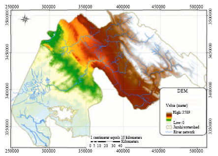 | |
| Fig. 2: | Dem and river network map of the study area |
The rainy season is limited to a 9 month period despite the continuous stream flow system (October-April). The mean annual precipitation is about 400 mm. Rain events usually last several days, although rainfall durations of 1 day or less do occur.
The used data was included monthly recorded rainfall from the rain-gauges of Mashregh, Shohada, Gorg, Shadegan and Shoe; Shadegan, Shoe temperature data and Mashregh, Behbahan and Gorg stream flow as well. Duration of these recorded data was 17 years from 1983-2000. A number of ANN models were designed and evaluated for their capability on stream flow prediction. Computational efficiencies of the GDX, CG and L-M algorithms and the effect of enabling/disabling of input parameters (various combinations of stream flow, rainfall and average air temperature) were also evaluated. This study started from January 2008 and completed in July 2009.
Data Preparation
Data on steam flow was limited to a 17 year period, then this period of record was used for model development by considering different combinations of inputs variables, e.g., rainfall, stream flow and average air temperature. For each one of the developed models available data were separated as 80% for training and 20% for validation. Additional analysis for the detection of network overtraining was not necessary in this research as the number of data points was more than the number of parameters used by the network (weights and biases). So, data could be divided into two parts for use in the training and validation stages, i.e., cross-validation analysis to stop overtraining was not required (Salehi et al., 2000). Data usage by an ANN model typically requires data scaling. This may be due to the particular data behavior or limitations of the transfer functions. For example, as the outputs of the logistic transfer function are between 0 and 1, the data are generally scaled in the range 0.1-0.9 or 0.2-0.8, to avoid problems caused by the limits of the transfer function (Maier and Dandy, 2000). In the present study, the data were scaled in the range of -1 to +1, based on the following equation:
| (4) |
Where:
| p0 | = | For the observed data |
| pn | = | Scaled data |
| pmax, pmin | = | For the maximum and minimum observed data points |
The above equation was used to scale average air temperature, as well stream flow and rainfall data in order to provide consistency of analysis. Then the unit of the scaled pn would correspond to individual data set (Burden et al., 1997) suggested that before any data preprocessing is carried out, the whole data set should be divided into their respective subsets (e.g., training and validation). In this study, the menu available in the Neural Network Toolbox of MATLAB were utilized for the normalization of the training data set, the transformation of the validation data set and the un-normalization of the network output, respectively. The routine normalizes the inputs and targets between -1 and 1, so that they will have zero mean and unit standard deviation. The validation data set was normalized with the mean and standard deviation, which were computed for the training data set. Finally, the network output was un-normalized and a regression analysis was carried out between the measured data and their corresponding un-normalized predicted data.
Evaluation Criteria for ANN Prediction
The performances of the ANN are measured with four efficiency terms. Each term is estimated from the predicted values of the ANN and the measured discharges (targets) as follows:
| • | The correlation coefficient (R-value) has been widely used to evaluate the goodness-of-fit of hydrologic and hydrodynamic models (Legates and Mccabe, 1999). This is obtained by performing a linear regression between the ANN-predicted values and the targets and is computed by: |
 | (5) |
Where:
| N | = | The number of samples |
| ti | = | Ti—T |
| pi | = | Pi—P |
| Ti and Pi | = | The target and predicted values for i = 1,….,N |
| = | The mean values of the target and predicted data set, respectively |
Note that a case with R is equal to 1 refers to a perfect correlation and the predicted values are either equal or very close to the target values, whereas there exists a case with no correlation between the predicted and the target values when R is equal to zero. Intermediate values closer to 1 indicate better agreement between target and predicted values (Maier and Dandy, 2000).
| • | The ability of the ANN-predicted values to match measured data is evaluated by the Root Mean Square Error (RMSE). It is defined as (Schaap and Leij, 1998) |
| (6) |
Overall, the ANN responses are more precise if R, MSE and RMSE are found to be close to 1, 0, 0 and 0, respectively. In the present study, MSE is used for network training, whereas R and RMSE are used in the network-validation phase.
Sensitivity Analysis
BPNN Structure Optimization
The crucial tasks in BP neural network modeling are to design a network with a specific number of layers, each having a certain number of neurons and to train the network optimally, so that it can map the system’s nonlinearity reasonably well. Some researchers stressed that optimal neural network design is problem-dependent and is usually determined by a trial- and -error procedure, i.e., sensitivity analysis (American Society of Civil Engineers or ASCE, 2000a, b).
Calibrations and Validations
In neural network methodology, learning, which extracts information from the input data, is a crucial step that is badly affected through (1) The selection of initial weights and (2) The stopping criteria of learning (Principe et al., 1999; Ray and Klindworth, 2000). If a well-designed neural network is poorly trained, the weight values will not be close to their optimum and the performance of the neural network will suffer. Little research has been conducted to find good initial weights (Haykin, 1999). In general, initial weight is implemented with a random number generator that provides a random value. In this study, the initial weights were randomly generated between -1 and 1 (Marinez and Martinez, 2005). To stop the training process, we could either limit the number of iterations or set an acceptable error level for the training phase.
There is no guarantee that coefficients which are close to optimal values will be found during the learning phase even though the number of iterations is capped at a predefined value. Therefore, to ensure that overtraining does not occur, we used three criteria to stop the training process; (1): RMSE is predefined and the training is conducted until the RMSE decreases to the threshold value. The idea is to let the system train until the point of diminishing returns, that is, until it basically cannot extract any more information from the training data. (2) Based on preliminary examinations, it was observed that the neural network error decreases as low as threshold RMSE within 100 epochs for good initial weights without overtraining; however, the threshold values may never be achieved for poor initial weights, even after a large number of epochs. (3) The minimum performance gradient (the derivatives of network error with respect to those weights and bias) is set to10 (Vos and Rientjes, 2005). The termination of the training process of the network is justified because the BPNN performance does not improve even if training continues. The training and validation procedures for specific network architectures were repeated in order to handle uncertainties of the initial weights and stopping criteria. In the preliminary investigation it was found that 10 trials were enough to find the best result. The performance efficiencies of each trial were recorded and compared. The result with the highest R-value of the training data set is considered the optimal ANN prediction for the network.
Another important task is the division of data for the network training and validation phase. The American Society of Civil Engineers (ASCE) Task Committee reported that ANNs are not very capable at extrapolation. Thus, in the present study, care was taken to have the training data include the highest as well as the lowest values, i.e., the two extreme input patterns. To ensure that the ANN is applicable to whole data set, about 40% of the total samples were chosen randomly from the rest of the data set for the validation phase. The stage and discharge records of the validation data are used for the rating curve prediction and comparison with ANN prediction.
Effect of Including Stream Flow Descriptive Data
The stream width and cross-sectional area at the measuring station do not change often, thus these can be easily estimated from the stream stage and the topography of the measuring station. However, it often posses a difficult task to continuously record the mean velocity of the stream. Therefore, the present study carried out the sensitivity analysis for three input data sets: average rain fall, average temperature and average steam flow to forecast monthly stream flows at Jarahi watershed.
RESULTS
Model Structures
Three model structures were developed to investigate the impact of variable enabling/disabling of input dimension on model performance. Model 1 is enabled for average temperature data as input dimension of two stations, model 2 is enabled for rain fall data as input dimension of five stations, model 3 is enabled for rainfall, average temperature and stream flow, Eq. 8-9 represent model 1 to Model 3, respectively.
| (7) |
| (8) |
| (9) |
Where:
| Q (t+1)sha deg an | = | Predicted rain fall-run off, for the time step of t+1 |
| {Qm, Qb, QGo} | = | Monthly rainfall-runoff data of Mashregh, Behbahan and Gorg hydrometric station |
| {PM, PShe, PSho, PSha, Pgo} | = | Monthly rainfall data of Mashregh, She, Shohada, Shadegan and Gorg rain gauge stations for the time step of t T (t)sho |
| T (t)sha | = | Average monthly air temperature data at Shohada and Shadegan station for the time step of t (Table 1) |
| Table 1: | Result of model performance level during training and validation stage |
 | |
 | |
| Fig. 3: | Comparison of predicated rainfall-runoff for the Calibrations and validations by different models; (a,a’) Model 1 (b,b’) Model 2 (c,c’) Model 3 |
Model Performance Levels
Table 1 shows individual model performance levels as measured by ERMS and R and individual model architecture as represented by the number of neurons in the input, output and hidden layers. Furthermore, computed rainfall-runoff by individual models are compared with the corresponding observed values and illustrated by their graph which is indicated by the results, it can be concluded that model 1 resulted with the lowest achieved performance levels. Disabling of Shohada, Shadegan stations rain gauge data, (model 2) resulted in a considerable improvement of the performance levels. Sheilan, Shohada, Shadegan, Gorge stations rain gauge (model 3) it is possible for the rainfall, average temperature and stream flow at the time of step t. Where, RMSE is root means squared error and R is correlation coefficient. In Fig. 3a-c are indicated a comparison of predicated rainfall-runoff by different models.
CONCLUSION
The Artificial Neural Network (ANN) models show an appropriate capability to model hydrological process. They are useful and powerful tools to handle complex problems compared with the other traditional models. In this study, the results show clearly that the artificial neural networks are capable of model rainfall-runoff relationship in the arid and semiarid regions in which the rainfall and runoff are very irregular, thus, confirming the general enhancement achieved by using neural networks in many other hydrological fields. In this research, the influences of training algorithm efficiencies and enabling/disabling of input dimension on rainfall-runoff prediction capability of the artificial neural networks was applied. A watershed system in Ahvaz area in the south region of Iran was used for the case study. The used data in ANN was monthly hydrometric and climatic data with 17 years duration from 1983-2000. For the mentioned model 14 year’s data were used for its development but for the validation/testing of the model 3 years data was applied. Three model structures were developed to investigate the probability impacts of enabling/disabling rainfall-runoff, rainfall, precipitation and the average air temperature input data. Efficiency of model 1 is enabled for average temperature data as input dimension with using two stations, model 2 for rain fall with using five stations and model 3 for rainfall, average temperature and stream flow data as input dimension with using six stations. Computational efficiencies, i.e., better achieved accuracy and convergence speed, were evaluated for the gradient descent (GDX), Conjugate Gradient (CG) and Levenberg-Marquardt (L-M) training algorithms. Since, the L-M algorithm was shown to be more efficient than the CG and GDX algorithm, therefore it was used to train the proposed tree models. Based on the results validation stage of Root Mean Square Error (RMSE) and coefficient of determination (r) measures were: 2.5, 0.47 (model 1); 1.57, 0.96 (model 2); 0.2, 0.998 (model 3). As indicated by the results, model 3 provided the highest performance. This was due to enabling of the rainfall, average temperature and stream flow data, resulting in improved training and thus improved prediction. The results of this study has shown that, with combination of computational efficiency measures and ability of input parameters which describe physical behavior of hydro-climatologic variables, improvement of the model predictability is possible in artificial neural network environment.
In general, ANN models applied to the rainfall-runoff transformation problem, show encouraging results according to the gained results of this study and the previous findings of (Dawson and Wilby, 1998; Hsu et al., 1995; Singh and Frevert, 2002a, b; Sajikumar and Thandaveswara, 1999; Smith and Eli, 1995; Tokar and Johnson, 1999; Tokar and Markus, 2000; Tan and Connor, 1996; Lee et al., 2002). Applying ANN to phenomena for which no adequate physically based models can be built, allows using these techniques in constructing hybrid models, with optimal combination of models of various types. The fact that ANNs exhibit a comparable or even better performance than a conceptual model suggests that this approach could provide a useful tool in solving similar type of problems in water resources studies and management (American Society of Civil Engineers or ASCE, 2000a, b; Hogue et al., 2006; Crawford and Burges, 2004).
These results presented in this study focused on the estimation of runoff discharge using the artificial neural network approach. This can be generalized to determine the flood hydrograph in the studied area. Here the Jarahi watershed in Iran is selected in this case study to demonstrate the application of the proposed technique. The distinct feature of this selected area is due to its geographical location and the limited rainfall-runoff data recorded from limited hydrologic stations. A feed-forward ANN is trained on the available historic data using the backward propagation algorithm.
ACKNOWLEDGMENTS
The author would like to thanks the Centre of Remote Sensing of the faculty of Natural Resources, University of Agriculture and Natural Research of Sari, Iran for financial and technical support. The author also thanks the reviewers for their constructive remarks.
REFERENCES
- Antcil, F. and N. Lauzon, 2004. Generalization for neural networks through data sampling and training procedures with applications to streamflow predictions. Hydrol. Earth Syst. Sci., 8: 940-958.
Direct Link - ASCE Task Committee on Application of Artificial Neural Networks in Hydrology, 2000. Artificial neural networks in hydrology. I: Preliminary concepts. J. Hydrol. Eng., 5: 115-123.
CrossRefDirect Link - ASCE Task Committee on Application of Artificial Neural Networks in Hydrology, 2000. Artificial neural networks in hydrology II: Hydrologic applications. J. Hydrol. Eng., 5: 124-137.
CrossRefDirect Link - Burden, F.R., R.G. Brereton and P.T. Walsh, 1997. Cross-validatory selection of test and validation sets in multivariate calibration and neural networks as applied to spectroscopy. Analysts, 122: 1015-1022.
PubMed - Hogue, T.S., H. Guptab and S. Sorooshian, 2006. A ‘user-friendly’ approach to parameter estimation J. Hydrol., 320: 202-217.
CrossRef - Chiang, Y.M., L.C. Chang and F.J. Chang, 2004. Comparison of static-feedforward and dynamic-fedback neural networks for rainfall-runoff modeling. J. Hydrol., 290: 297-311.
CrossRef - Crawford, N.H. and S. J. Burges, 2004. History of the Stanford watershed model. Water Resour. IMPACT, 6: 3-5.
Direct Link - Vos N.J.D. and T.H.M. Rientjes, 2005. Constraints of artificial neural networks for rainfall-runoff modeling trade-offs in hydrological state representation and model evaluation. Hydrol. Earth Syst. Sci., 9: 111-126.
Direct Link - Gautam, M.R., K. Watanabe and H. Saegusa, 2000. Runoff analysis in humid forest catchment with artificial neural network. J. Hydrol., 235: 117-136.
Direct Link - Hsu, K.L., H.V. Gupta and S. Sorooshian, 1995. Artificial neural network modeling of the rainfall-runoff process. Water Res. Res., 31: 2517-2530.
Direct Link - Jain, A., K.P. Sudheer and S. Srinivasulu, 2004. Identification of physical processes inherent in artificial neural network rainfall-runoff models. Hydrol. Process., 118: 571-581.
Direct Link - Kitanidis, P.K. and R.L. Bras, 1980. Adaptive filtering through detection of isolated transient errors in rainfall-runoff models. Water Resour. Res., 16: 740-748.
CrossRefDirect Link - Kitanidis, P.K. and R.L. Bras, 1980. Real-time forecasting with a conceptual hydrological model. Water Resour. Res., 16: 1025-1033.
Direct Link - Lee, D.S., C.O. Jeon, J.M. Park and K.S. Chang, 2002. Hybrid neural network modeling of a full-scale industrial wastewater treatment process. Biotechnol. Bioengin., 78: 670-682.
CrossRefDirect Link - Legates, D.R. and G.J. Mccabe, 1999. Evaluating the use of goodness-of-fit measures in hydrologic and hydro-climatic model validation. Water Resour. Res., 35: 233-241.
Direct Link - Maier, H.R. and G.C. Dandy, 2000. Neural networks for prediction and forecasting of water resources variables a review of modeling issues and applications. Environ. Model. Software, 15: 101-124.
Direct Link - O'Connell, P.E., J.E. Nash and J.P. Farrell, 1970. River flow forecasting through conceptual models part II-The Brosna catchment at Ferbane. J. Hydrol., 10: 317-329.
CrossRefDirect Link - Rajurkar, M.P., U.C. Kothyari and U.C. Chaube, 2004. Modeling of daily rainfall-runoff relationship with artificial neural network. J. Hydrol., 285: 96-113.
Direct Link - Rumelhart, D.E., G.E. Hinton and R.J. Williams, 1986. Learning representations by back-propagating errors. Nature, 323: 533-536.
Direct Link - Ray, C. and K.K. Klindworth, 2000. Neural networks for agrichemical vulnerability assessment of rural private wells. J. Hydrol. Eng., 5: 162-171.
Direct Link - Salehi, F., S.O. Prashar, S. Amin, A. Madani and S.J. Jebelli et al., 2000. Prediction of annual nitrate-N losses in drain out.ows with artificial neural networks. Trans ASAE., 43: 1137-1143.
Direct Link - Schaap, M.G. and F.J. Leij, 1998. Database related accuracy and uncertainty of pedotransfer functions. Soil Sci., 163: 765-779.
Direct Link - Sajikumar, N. and B.S. Thandaveswara, 1999. A non-linear rainfall-runoff model using an artificial neural network. J. Hydrol., 216: 32-55.
Direct Link - Sudheer, K.P. and A. Jain, 2004. Explaining the internal behavior of artificial neural network river flow model. Hydrol. Process., 118: 833-844.
Direct Link - Smith, J. and R.N. Eli, 1995. Neural-network models of rainfall-runoff process. J. Water Res. Plan. Manage., 121: 499-508.
Direct Link - Tokar, A.S. and P.A. Johnson, 1999. Rainfall-runoff modeling using artificial neural network. J. Hydrrol. Eng., 4: 232-239.
Direct Link - Tan, B.Q. and K.M.O. Connor, 1996. Application of an empirical infiltration quation in the SMAR conceptual model. J. Hydrol., 185: 275-295.
Direct Link - Tokar, A.S. and M. Markus, 2000. Precipitation-runoff modeling using artificial neural networks and concettual models. J. Hydrol. Eng., 5: 156-161.
Direct Link - Wilby, R.L., R.J. Abrahart and C.W. Dawson, 2003. Detection of conceptual model rainfall-runoff processes inside an artificial neural network. Hydrol. Sci. J., 48: 163-181.
Direct Link - Zhang, B. and R.S. Govindaraju, 2003. Geomorphology-based artifical neural networks (GANNs) for estimation of direct runoff over watersheds. J. Hydrol., 273: 18-34.
CrossRef - Cannon, A.J. and P.H. Whitfield, 2002. Downscaling recent streamflow conditions in British Columbia, Canada using ensemble neural network models. J. Hydrol., 259: 136-151.
CrossRef - Shamseldin, A.Y., 1997. Application of a neural network technique to rainfall-runoff modelling. J. Hydrol., 199: 272-294.
CrossRefDirect Link