
B.J. Alsulayfani
Department of Civil Engineering, College of Engineering, University of Mosul, Iraq
T.E. Saaed
Department of Civil Engineering, College of Engineering, University of Mosul, Iraq
Asian Journal of Applied Sciences
Year: 2009 | Volume: 2 | Issue: 4 | Page No.: 348-362


ABSTRACT
The aim of this study is to determines the effects of methods of analysis used in the analysis and design of high rise steel buildings. As it known, many methods are available for the structural analysis of buildings and other civil engineering structures under seismic actions. The differences between them lie in the way they incorporate the seismic input and in the idealization of the structure. There are two procedures for specifying seismic design forces: first, the equivalent static force and second, the dynamic analysis which can take a number of forms. Mode superposition is one of these forms. Design codes have proposed different formulas to obtain a more reasonable estimate of the maximum response from the spectral values (SRSS, CQC, ASCE-98, TEN, ABS, CSM). This research studies the effect of these formulas in the analysis and design of high rise reentrant steel buildings. The study then compares the resulting steel sections weight using static and dynamic analysis, the latter being by means of mode combination methods to show the difference between these formulas, to determine the most influenced structural members and to obtain the vertical loads factor in order to get the required sections using common static analysis for preliminary design purposes. The study shows that modal combination methods slightly affect the result of design for building; the difference among the formulas does not exceed more than 2.5%. The columns especially those at lower floors are mainly affected by seismic forces, while the beams are slightly affected. Finally, a factor of (10.5%) of the total vertical loads (excluding self weight of the building) can be used to predict the members sections, instead of dynamic analysis which is time consuming even with high speed computers like those used in this research.
PDF Abstract XML References Citation
How to cite this article
B.J. Alsulayfani and T.E. Saaed, 2009. Effect of Dynamic Analysis and Modal Combinations on Structural Design of Irregular High Rise Steel Buildings. Asian Journal of Applied Sciences, 2: 348-362.
DOI: 10.3923/ajaps.2009.348.362
URL: https://scialert.net/abstract/?doi=ajaps.2009.348.362
DOI: 10.3923/ajaps.2009.348.362
URL: https://scialert.net/abstract/?doi=ajaps.2009.348.362
INTRODUCTION
According to Naiem (1989) in order to design a structure to withstand an earthquake, the forces on the structure must be specified. The exact forces that will occur during the life of the structure cannot, of course, be known. Many methods are available for the structural analysis of buildings and other civil engineering structures under seismic actions. The differences between the methods lie in the way they incorporate the seismic input and in the idealization of the structure. There are two commonly used procedures for specifying seismic design forces. The equivalent static force procedure and dynamic analysis. In the equivalent static force procedure the inertial forces are specified as static forces using empirical formulas. The empirical formulas do not explicitly account for the dynamic characteristics of the particular structure being designed or analyzed. The formulas were, however, developed to adequately represent the dynamic behavior of what are called regular structures which have a reasonably uniform distribution of mass and stiffness. For such structures the equivalent static force procedure is often adequate.
Structures that do not fit into this category are termed irregular. Common irregularities include large floor to floor variation in mass or center of mass and soft stories. Such structures violate the assumptions on which the empirical formulas used in the equivalent static force procedures are based. Therefore, its use may lead to erroneous results. In these cases a dynamic analysis should be used to specify and distribute the seismic design forces. A dynamic analysis can take a number of forms, but should take account of the irregularities of the structure by modeling its dynamic characteristics including natural frequencies, mode shapes and damping (Naiem, 1989).
According to Edward (2002) the mode displacement super-position method provides an efficient means of evaluating the dynamic response of most structures because the response analysis is performed only for a series of SDOF systems. The response analysis for the individual modal equations requires very little computational effort and in most cases only a relatively small number of the lowest modes of vibration need to be included in the superposition. With this regard, it is important to realize that the physical properties of the structure and the characteristics of the dynamic loading generally are known only approximately; hence, the structural idealization and the solution procedure should be formulated to provide only a corresponding level of accuracy. Nevertheless, the mathematical models developed to solve practical problems in structural dynamics range from very simplified systems having only a few degrees of freedom to highly sophisticated finite element models including hundreds or even thousands of degrees of freedom in which as many as 50 to 100 modes may contribute significantly to the response (Edward, 2002).
The basic mode superposition method, which is restricted to linearly elastic analysis, produces the complete time history response of joint displacements and member forces. The method involves the calculation of only the maximum values of the displacements and member forces in each mode using smooth design spectra that are the average of several earthquake motions.
Generally, maximum total response cannot be obtained by merely adding the modal maxima because these maxima usually do not occur at the same time. In most cases, when one mode achieves its maximum response, the other modal responses are less than their individual maxima. Therefore, although the superposition of the modal spectral values obviously provides an upper limit to the total response, it generally over estimates this maximum by a significant amount. A number of different formulas have been proposed to obtain a more reasonable estimate of the maximum response from the spectral values (Edward, 2002):
| • | SRSS (square root of the sum of squares ) |
| • | CQC (the complete quadratic combination) |
| • | ASCE4-98 (ASCE) |
| • | TEN the 10% |
| • | ABS (the absolute) |
| • | CSM (closely-spaced mode) |
This research studies the effect of these approaches on the analysis and design of high rise reentrant steel buildings. It compares the resulting steel sections weight using static and dynamic analysis utilizing mode combination methods approaches to show the difference among these approaches, to determine the most influenced structural members and to obtain a vertical loads factor in order to get the required sections using common static analysis for preliminary design purposes.
DYNAMIC EQUILIBRIUM
The force equilibrium of a multi-degree-of-freedom lumped mass system as a function of time can be expressed by the following relationship (Edward, 2002; Ray and Penzien, 2003):
| F (t)I+F (t)D+F (t)S = F (t) | (1) |
in which the force vectors at time t are:
| F (t)I | = | Vector of inertia forces on the node masses |
| F (t)D | = | Vector of viscous damping or energy dissipation, forces |
| F (t)S | = | Vector of inernal forces carried by the structure |
| F (t) | = | Vector of externally applied loads |
Equation 1 is based on physical laws and is valid for both linear and nonlinear systems if equilibrium is formulated with respect to the deformed geometry of the structure. For many structural systems, the approximation of linear structural behavior is made to convert the physical equilibrium statement, Eq. 1, to the following set of second-order, linear, differential equations:
| | (2) |
where, M is the mass matrix (lumped or consistent), C is a viscous damping matrix (which is normally selected to approximate energy dissipation in the real structure) and K is the static stiffness matrix for the system of structural elements. The time-dependent vectors ![]() and
and ![]() are the absolute node displacements, velocities and accelerations, respectively.
are the absolute node displacements, velocities and accelerations, respectively.
For seismic loading, the external loading F(t) is equal to zero. The basic seismic motions are the three components of free-field ground displacements u (t)ig that are known at some point below the foundation level of the structure. Therefore, we can write Eq. 2 in terms of the displacements ![]() , velocities
, velocities ![]() and accelerations
and accelerations ![]() that are relative to the three components of free-field ground displacements. Therefore, the absolute displacements, velocities and accelerations can be eliminated from Eq. 2 by writing the following simple equations:
that are relative to the three components of free-field ground displacements. Therefore, the absolute displacements, velocities and accelerations can be eliminated from Eq. 2 by writing the following simple equations:
 | (3) |
where, Ii is a vector with ones in the i directional degrees-of-freedom and zero in all other positions. The substitution of Eq. 3 into Eq. 2 allows the node point equilibrium equations to be rewritten as:
| | (4) |
where, Mi = MIi
The simplified form of Eq. 4 is possible since the rigid body velocities and displacements associated with the base motions cause no additional damping or structural forces to be developed.
There are several different classical methods that can be used for the solution of Eq. 4. Each method has advantages and disadvantages that depend on the type of structure and loading. The different numerical solution methods are :
| • | Step-by-step solution method |
| • | Mode superposition method |
| • | Response spectra analysis |
| • | Solution in the frequency domain |
| • | Solution of linear equations |
| • | Undamped harmonic response |
| • | Undamped free vibrations |
The most common and effective approach for seismic analysis of linear structural systems is the mode superposition method. After a set of orthogonal vectors have been evaluated, this method reduces the large set of global equilibrium equations to a relatively small number of uncoupled second order differential equations. The numerical solution of those equations involves greatly reduced computational time. The dynamic force equilibrium, Eq. 4 can be rewritten in the following form as a set of Nd second order differential equations:
| | (5) |
All possible types of time-dependent loading, including wind, wave and seismic, can be represented by a sum of J space vectors fj, which are not a function of time and J time functions g (t)j.
The fundamental mathematical method that is used to solve Eq. 5 is the separation of variables. This approach assumes the solution can be expressed in the following form:
| | (6a) |
where, Ø is an Nd by N matrix containing N spatial vectors that are not a function of time and Y(t) is a vector containing N functions of time. From Eq. 6a, it follows that:
| | (6b) |
| | (6c) |
Before solution, we require that the space functions satisfy the following mass and stiffness orthogonality conditions:
| | (7) |
where, I is a diagonal unit matrix and Ω2 is a diagonal matrix in which the diagonal terms are ![]() . The term ωn has the units of radians per second and may or may not be a free vibration frequencies. It should be noted that the fundamentals of mathematics place no restrictions on those vectors, other than the orthogonality properties. In this research each space function vector, Φn, is always normalized so that
. The term ωn has the units of radians per second and may or may not be a free vibration frequencies. It should be noted that the fundamentals of mathematics place no restrictions on those vectors, other than the orthogonality properties. In this research each space function vector, Φn, is always normalized so that ![]() .
.
The generalized mass is equal to one, or after substitution of Eq. 6 into Eq. 5 and the pre-multiplication by ΦT, the following matrix of N equations is produced:
| | (8) |
where, Pj = ΦT fj and are defined as the modal participation factors for load function j. The term Pnj is associated with the nth mode. Note that there is one set of N modal participation factors for each spatial load condition fj. For all real structures, the N by N matrix d is not diagonal; however, to uncouple the modal equations, it is necessary to assume classical damping where there is no coupling between modes. Therefore, the diagonal terms of the modal damping are defined by:
| | (9) |
where, ζn is defined as the ratio of the damping in mode n to the critical damping of the mode. A typical uncoupled modal equation for linear structural systems is of the following form:
| | (10) |
For three-dimensional seismic motion, this equation can be written as:
| | (11) |
where, the three-directional modal participation factors, or in this case earthquake excitation factors, are defined by ![]() , where, j is equal to x, y or z and n is the mode number. Note that all mode shapes are normalized so that
, where, j is equal to x, y or z and n is the mode number. Note that all mode shapes are normalized so that ![]() .
.
For three-dimensional seismic motion, the typical modal Eq. 11 is rewritten as:
| | (12) |
where, the three mode participation factors are defined by ![]() , which i is equal to x, y or z. Two major problems must be solved to obtain an approximate response spectrum solution to this equation. First, for each direction of ground motion, maximum peak forces and displacements must be estimated. Second, after the response for the three orthogonal directions has been solved, it is necessary to estimate the maximum response from the three components of earthquake motion acting at the same time.
, which i is equal to x, y or z. Two major problems must be solved to obtain an approximate response spectrum solution to this equation. First, for each direction of ground motion, maximum peak forces and displacements must be estimated. Second, after the response for the three orthogonal directions has been solved, it is necessary to estimate the maximum response from the three components of earthquake motion acting at the same time.
STRUCTURE ANALYSIS AND DESIGN
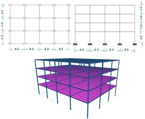
A reentrant steel building consisting of twenty stories, shown in Fig. 1 and 2, has been analyzed using STAAD PRO 2007 software for dynamic analysis under the following loads:
| • | Self weight |
| • | Finish loads = 4.9 kN m-2 |
| • | Live loads = 2 kN m-2 |
| • | UBC 1985 code according to STAAD PRO 2007 function |
| • | Element load = DL+25% LL |
| • | Element load = 4.9 (FL) +0.25x2.0 (LL) = 6.4 kN m-2 |
| • | Response spectra according to STAAD PRO 2007 function |
Then combinations of loads including checker board pattern have been done as shown in Table 1, taking into consideration the effect of seismic forces (as equivalent static force and response spectra forces for the only first five modes), the coefficients used in seismic analysis are shown in Table 2-4 and 6, also P-delta analysis has been done.
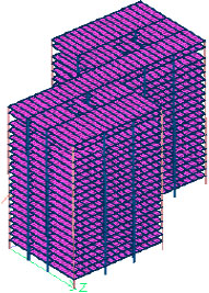 | |
| Fig. 1: | Building 3D view |
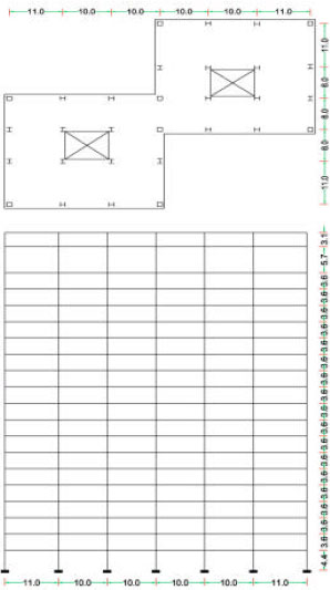 | |
| Fig. 2: | Building plan and section |
| Table 1: | Load cases used in analysis and design of building |
 | |
 | |
 | |
| Table 2: | UBC factors used in analysis |
 | |
| Table 3: | Response spectrum factors used in analysis |
 | |
| Table 4: | Response spectra used in analysis and design |
 | |
Then the structural design of members was carried out to select members sections, which were in turn organized in groups for each floor as shown in Table 5 and Fig. 3, 4 to obtain the optimum steel sections weight. Six modal combination approaches are used for analysis, namely (SRSS, CQC, ASCE-98, TEN, ABS, CSM) to predict the difference in design among them. Also analysis was carried out for the building in case of using equivalent static force only and for common static analysis, to predict the difference in steel sections weights.
 | |
 | |
| Fig. 3: | Design group for first storey |
 | |
 | |
| Fig. 4: | Design group for 10th and 20th storey |
| Table 5: | Members groups description |
 | |
RESULTS AND DISCUSSION
The results are shown in Fig. 5. It is obvious that ABS approaches differ from other approaches of modal combinations. While SRSS and CQC provided values that are slightly differs and in good agreement with Amr et al. (2008).
Table 6 shows the weight of steel sections and percentage of steel weight relative to static method for the entire building according to methods of structural analysis. In Table 7, the weight of columns steel sections for selected stories of building according to their locations and methods of analysis is shown. While in Table 8 the weight of beams steel sections for selected stories of building according to their locations and methods of analysis is shown also.
Common static and UBC analysis under estimate the design. Figure 6 and 7 show that the columns, especially those at the lower floors, are influenced with analysis type more than beams. For this reason the building has been analyzed (common static analysis only) and designed for several percentage increments in total vertical loads to get the percentage at which the same weight of steel section can be obtained, compared to dynamic analysis. In Fig. 8, it is obvious that this percentage is (10.5% ).
This percentage (10.5%) has been used to analyze and design two other buildings under the same conditions and load cases to show whether this percentage is correct or not.
Figure 9 shows the plan and section of building No. 1. Total steel sections weight obtained under dynamic loads was (900.2 kN), while the total steel sections weight under common static analysis with vertical loads multiplied by the factor (10.5%) was (906.4 kN). This indicates that the factor (10.5%) is correct.
Figure 10 shows the plan and section of building No. 2. In this case, the total steel sections weight obtained under dynamic loads was (912 kN), whereas, the total steel sections weight under common static analysis with vertical loads multiplied by the factor (10.5%) was (868 kN). This indicates that the factor (10.5%) is correct for this case also and can be used for preliminary design purposes.
| Table 6: | Weight of steel sections for the entire building according to methods of structural analysis |
 | |
| Table 7: | Weight of columns steel sections for selected stories of building according to their locations and methods of analysis |
 | |
| Table 8: | Weight of beams steel sections for selected stories of building according to their locations and methods of analysis |
 | |
 | |
| Fig. 5: | Relation between type of structural analysis and total weight of steel sections |
 | |
| Fig. 6: | Effect of structural analysis type on columns steel sections weight |
 | |
| Fig. 7: | Effect of structural analysis type on beams steel sections weight |
 | |
| Fig. 8: | Percent of total vertical loads increment and designed steel sections weight |
 | |
| Fig. 9: | Building No. 1 plan, section and 3D view |
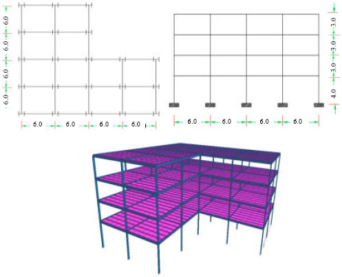 | |
| Fig. 10: | Building No. 2 plan, section and 3D view |
NOMENCLATURE
| F(t)I | : | A vector of inertia forces on the node masses |
| F(t)D | : | A vector of viscous damping, or energy dissipation, forces |
| F(t)S | : | A vector of inernal forces carried by the structure |
| F(t) | : | A vector of externally applied loads |
| M | : | The mass matrix (lumped or consistent) |
| C | : | A viscous damping matrix |
| K | : | The static stiffness matrix |
| u(t)a | : | Vector are the absolute node displacements |
| : | Vector are the absolute node velocities | |
| ü(t)a | : | Vector are the absolute node accelerations |