
Zouhir Wakaf
King Saud University, Saudi Arabia
Mariam M. Saii
Taif University, Saudi Arabia
Research Journal of Information Technology
Year: 2009 | Volume: 1 | Issue: 1 | Page No.: 17-29


ABSTRACT
A system for face recognition in colored frontal face images is proposed. This study presents a new scheme for feature extraction based on deformable models and morphs using the 2D wavelet multi-resolution decomposition, then, a classical semi-parametric system of a multi layered perceptron neural network is employed for classification purpose. A heuristic is designed for defining the face only bounding rectangle thus excluding most of the facial hair, ears and neck and then we defined depending on this computed rectangle four regions of interest, representing the forehead, eye`s sockets, nose and chin regions. This heuristic also gives our system invulnerability against both translations and z-axis limited rotations. Next, 2D wavelet coefficients for the three channels of red, green and blue are computed for the whole image using the multi-resolution decomposition. A classification system of back propagation multi layered perceptron neural network is designed and trained with momentum learning and the cross validation during network training in the search procedure and the hyper tangent nonlinearity as an activation function. Our system is experimented with colored faces from the Stirling University database and the preliminary results we obtained show an 88% success rate.
PDF Abstract XML References Citation
How to cite this article
Zouhir Wakaf and Mariam M. Saii, 2009. Frontal Colored Face Recognition System. Research Journal of Information Technology, 1: 17-29.
URL: https://scialert.net/abstract/?doi=rjit.2009.17.29
URL: https://scialert.net/abstract/?doi=rjit.2009.17.29
INTRODUCTION
The problem of face recognition was considered in the early stages of computer vision and is now undergoing a revival after nearly 20 years. Different specific techniques were proposed or reprocessed recently (Wu and Huang, 1990; Nakamura et al., 1991; Golomb et al., 1991). In recent years, the growing demand for reliable automatic personal identification systems has resulted in an increased interest in biometric researches. Biometrics includes fingerprint recognition, speech recognition, signature dynamics and of course face recognition.
Although face recognition among the rest of the recognition techniques has the benefit of being a passive and non-intrusive way for identity verification, however, human faces represent very complex, multi-dimensional visual stimuli and developing a computational model for face recognition is very difficult. In order to achieve a feasible practical systems some constraints should be set, in our case, these constraints are frontal pose under minor variations of lighting and scale.
In addition to the previously mentioned constraints, the successful implementation of the system also depends on the application it is being used for. So, we can identify at least two broad categories of frontal face recognition systems:
| • | Off-line face recognition systems: The objective of those systems is to find a person within a large database of faces (e.g., in a police criminal database). These systems typically return a list of the most likely people in the database. Often only one image available per person and it`s usually not necessary for the recognition to be done in real-time. |
| • | On-line face recognition systems: Here the objective is to identify particular people in real-time (e.g., security monitoring system, or location tracking system, etc.), or we want to allow access to a group of people and deny access to all the other. Multiple images per person are often available for training and real-time recognition is required. |
In this study, we are primarily interested in the first case. We are also interested in recognizing frontal faces with various facial expressions, facial transitions, z-axis head rotations within the range of ± 10 ° and facial details. We do not consider the extreme facial translations nor the head rotations more than 10 ° nor the vast variations of illumination or scale. We tested the efficiency and the effectiveness of our system on the Stirling University database of colored faces, which is composed of high-resolution images with an average of (330x440) pixels, such large samples are considered non-practical to use in many other systems of face recognition.
THE FACE RECOGNITION SYSTEM
Our proposed new hybrid system consists from three stages as shown in the block diagram of Fig. 1. The Face Recognition System stages are:
Input Stage
For acquiring colored face images from any online connected cameras, scanners, or from stored image files (BMPs, GIFs, JPEGs, TIFFs, etc...).
Face Locating and Feature Extraction Stage
In order to realize human-like image recognition system and to allow queries at a higher semantic level, some particular pictorial objects have to be detected and exploited for indexing, that is to say Extract Features. In recent years, considerable progress has been made on the problem of face feature extraction for later detection and recognition (Wilson et al., 1994; Dai and Nakano, 1998; Daubechies, 1990; Brunelli and Paggio, 1992). These methods can be roughly divided into two different groups: geometrical features matching and template matching. In the first case, some geometrical measures about distinctive facial features such as eyes, mouth, nose and chin are extracted (Brunelli and Paggio, 1993). In the second case, the face image, represented as a two-dimensional array of intensity RGB values, is compared to a single or several templates representing a whole face.
In this study, we propose a new method for face feature extraction based on a 2-D wavelet decomposition of the face images. Each face image is described by a subset of band filtered images containing wavelet coefficients for the 3 channels RGB.
 | |
| Fig. 1: | The Block diagram of the proposed colored frontal face recognition system |
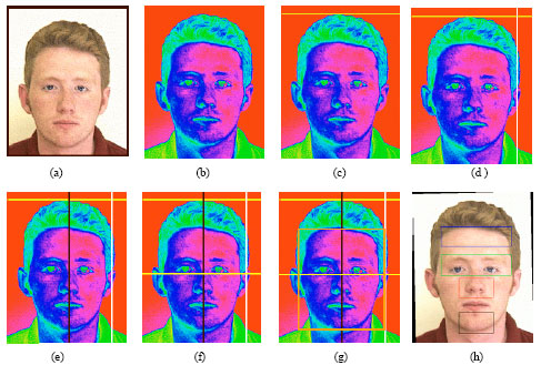 | |
| Fig. 2: | The feature extraction stages. The original is colored image, (a) the original image, (b) the outcome Pseudo Color transform, (c) the head`s top, (d) the first left side skin texture, (e) the face’s vertical center, (f) the left eye down edge, (g) the final bounding rectangle of the face and (h) the four regions of interest |
From these wavelet coefficients, which characterize the face texture and outlay, we form compact and meaningful feature vectors, using simple statistical measures (coefficient`s mean values and the deviation values). This stage itself consists of the following steps:
Step 1: Image Preprocessing Section
Some digital image processing filters is applied to normalize the face images as much as possible, thus reducing any unwanted noise or minor illumination variations (Fig. 2a).
Step 2: Transform a Colored Image into a Pseudo Color
The colored face image is transformed into a pseudo-color one, from which it can extract the overall face from the homogenous background of white or black. What this transform do is set the pixel colors of the image to, red, green and blue or to their dual combinations of cyan, magenta and yellow according to the pixel`s current palette values. Figure 2b shows outcome of this transform.
Step 3: Locate the Top Head and First Left Side of the Image
The first occurrence of the non-background is located, when doing a descending scan of the pseudo-color image in order to locate the top of the head in the image. Then we try locating the first left side occurrence of facial skin texture compared to the homogenous background, we take advantage of red and blue colors (purple intensities at any selected pixel), as follows (pseudo code). Figure 2c and d, show the top head and the first side skin texture in the image of the face, respectively.
Step 4: Locate the Vertical Center of the Face
At this current stage and after we defined and located top and left boundaries of the face, it`s possible using a deformable template matching to define precisely the vertical center of the face. Deformable template is a common method used in detecting facial features (Yuille et al., 1992). The result we obtained using a (180x200) pixel template are shown in Fig. 2e.
Step 5: Face Region Detection
After locating the vertical center, we can define the width of the bounding rectangle. But it is much better finding the onset rectangle`s height and then we can define the rectangle as whole. For achieving this we try to find the lower edge of the left eye which should be trivial matter now, then we had found both the vertical center of the face and the leftmost boundary of the face. In this step also we seek the down edge of the other eye from which we can find if the two eyes lay on the same horizontal distance from the top of the image, thus finding if the face is rotated or not, if so we can cancel this rotation affect (the plane z-axis rotations only).
Since the other two axis rotations y-axis and x-axis are considered as profile face and a view tolerant in the later case. Although in this step and in the heuristic in general can detect z-axis rotations more than ± 10° it is not implemented, because we consider such images to be non-valid pattern samples. Figure 2f and g, show the result of this step.
Step 6: Region of Interest Detection
After we had outlined the bounding rectangles we can define more strict regions of interest for a given pattern (face image) within those rectangles, thus, reducing the dimensionality of the problem at hand and at the same time conserving the accuracy.
We chose four regions of interest. The regions are forehead, eyes, nose and the chin region as shown in Fig. 2h.
We didn`t include the mouth because it is one of those non-rigid features of the face, which is highly affected by facial expressions.
2D Wavelet Multi-Resolution Decomposition
Images are represented as a two-dimensional array of coefficients, each coefficient representing the brightness level in that point. When looking from a higher perspective, we can`t differentiate between coefficients as more important ones and lesser important ones. But thinking more intuitively, we can. Most natural images have smooth color variations, with the fine details being represented as sharp edges in between the smooth variations. Technically, the smooth variations in color can be termed as low frequency variations and the sharp variations as high frequency variations.
The low frequency components (smooth variations) constitute the base of an image and the high frequency components (the edges which give the detail) add upon them to refine the image, thereby giving a detailed image. Hence, the smooth variations are demanding more importance than the details.
Separating the smooth variations and details of the image can be done in many ways. One such way is the decomposition of the image using a 2D wavelet multi-resolution decomposition. The 2D wavelet Multi-Resolution Decomposition (MRD) (Daubechies, 1990) has been proven effective for image analysis and feature extraction. It represents a signal by localizing it in both time and frequency domains.
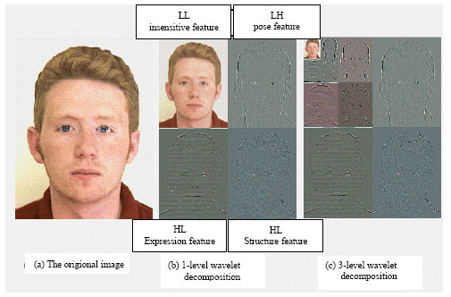
Next, the filtering is done for each column of the intermediate data. The resulting two-dimensional array of coefficients contains four bands of data, each labeled as LL (low-low), HL (high-low), LH (low-high) and HH (high-high). The LL band can be decomposed once again in the same manner, thereby producing even more sub bands. This can be done up to any level, thereby resulting in a pyramidal decomposition as shown in Fig. 3.
Figure 4 shows the decomposition process by applying the 2D wavelet transform on a face image. The original image shown in Fig. 4a is decomposed into four sub band images shown in Fig. 4b. Similarly, we can obtain 3 levels of the Wavelet decomposition as shown Fig. 4c by applying wavelet transform on the low frequency band sequentially.
 | |
| Fig. 3: | The 2D multi-resolution decomposition of an image. (a) Single level, (b) two levels and (c) three level decompositions |
 | |
| Fig. 4: | The four regions of interest from which we are going to compute the means and the variances |
Extracting Sub Band Feature Vector
In order to achieve the dimensionality reduction, we first decided that for the image`s size on which we experimented, performing a 3 level decomposition for each face is adequate (usually an entropy-based criterion is used to determine the best decomposition level) (Lin and Wu, 1999). There is no need to perform a deeper decomposition because after the third level, the size of the image becomes too small and no more valuable information is obtained. At the third level of decomposition, we obtain one image of approximation (low frequency image) and nine of details for each channel (RGB). Therefore, the face image is described by 30 wavelet coefficient matrices (3n+1 where n corresponds to the decomposition number).
At the current point we have performed a 3 level wavelet decomposition using Daub4 wavelet and we have 30 wavelet coefficient matrices.
Next, for each sub band LL, LH, HL except for sub band HH of the 3 levels, we are going to calculate the mean and the variance of their coefficients as following:
| • | For each sub band except HH sub bands of every level, we will consider only those coefficients which are located within the predefined 4 regions of interest. |
| • | We will compute both the mean and variance of the 1 level LL sub band and for the 3 channels red, green and blue. This produces the first 24 vector values we are going to use in the classification stage. |
| • | For all the LH sub bands in the 3 levels, we will compute the variance of its coefficients for the 3 channels of RGB in 3 regions only, for the forehead, eyes and the chin regions. This yields a total of 27 vectors. |
| • | For all the HL sub bands in the 3 levels, we will compute the variance of its coefficients for the 3 channels of RGB in 2 regions only, for the eyes and the nose regions. This gives a total of 18 vectors. |
With this final step we conclude our feature extraction system, from which we had a total of 69 vectors representing the mean and the variances of the different sub bands in the 3 level decomposition within a predefined interest regions. The mean and the variance can be computed using the following formulas:
(1) |
And the vectors to be used as an input for the next stage are:
(2) |
where, μi the mean value for last level coefficient matrices is, σ2j is the variance for the matrices of all level decompositions considered.
We also must note that, calculating the variances and the means of the sub band`s coefficients in those predefined regions, corresponds to producing global measurements of the texture and intensity values of those regions.
Face Recognition
A backpropagation neural network is used for the recognition purpose with the momentum learning deploys because it speeds up and stabilizes the learning during the training phase (Juell and Marsh, 1996; Lawrence et al., 1997). From Block diagram shown in Fig. 5, this topology consists of:
| • | Input buffer layer of 69 neurons (processing elements), which are all fully connected to all the neurons of the hidden layer. |
| • | One hidden layer of 46 neuron, with the following common parameters for all its neurons: Step size η = 1.4, momentum rate α = 0.7, weight variances = ± 0.6, bias variances = ± 0.5, activation function (squashing function) = Sigmoid Function, all the neurons are fully connected to all the neurons in the output layer. |
| • | Output layer of 12, 18, 24 neuron (since we have experimented on 12, 18, 24 different patterns or persons), with the following parameters common for all its neuron: step size η = 0.6, momentum rate α = 0.7, weight variances = ± 0.2, bias variances = ± 0.5, activation function (squashing function) = Sigmoid Function. |
All training sample pattern`s feature vectors were normalized prior to be presented to the network according to the following relation:
 | |
| Fig. 5: | The block diagram of a one hidden layer backpropagation neural network, which is used in the classification stage |
(3) |
where, maxValue R2 = 0.998877, min Value R2 = 0.112233, maxValueR1, minValue R1 are the maximum and minimum values for all the vectors with same index in all training samples.
All the output target values for the previous input samples were initialized as following: all the outputs (12, 18 and 24) set to 0.112233 except for the output that corresponds to the target pattern, it was set to 0.998877. For instance, if a pattern X, is located forth in the pattern database, then it will have the pattern number 3 and thus its output target values will be:
{0.112233, 0.112233, 0.112233, 0.998877, 0.112233, 0.112233, 0.112233, 0.112233, 0.112233, 0.112233, 0.112233, 0.112233, 0.112233, 0.112233, 0.112233, 0.112233, 0.112233, 0.112233, 0.112233, 0.112233, 0.112233, 0.112233, 0.112233, 0.112233}. |
All the weights and the biases are initialized with random values within a range defined according to the weight and bias variances for the hidden and the output layers.
We preferred the on-line learning approach over the batch learning, for the later requires more processing and memory resources as it updates the weights after presenting all the sample patterns to the network while accumulating the errors. In the on-line learning case weights update takes place after presenting each pattern, but here we must shuffle the sample patterns every epoch to ensure that the network won`t forget the last pattern it was presented with and eventually stall. The neural network will be trained for a number of epochs, until the final error gets less than a predefined value usually less than 0.01.
In the test phase, the tested sample patterns will be first normalized against all the patterns in the database and then they will be propagated forward in the network and the corresponding output will be compared with the stored pattern`s outputs database.
RESULTS AND DISCUSSION
The experimental results are described here and the ups and downfalls of each stage are discussed.
First, we will start with face locating and rectangle defining stage: As we stated stage 2 locates the face and define the 4 regions of interest under various variations of facial translations and rotations, next is the experimental results of its capabilities.
Figure 6-10 show the capabilities of our proposed heuristic for detecting face translations and z-axis only rotations.
We tried our heuristic on all the images we experimented on and it successfully located and defined all of them.
Second, we present the experimental results of the third section of the second stage, where we deployed the 2D wavelet multi-resolution decomposition for feature extraction.
Figure 10 Show the feature vectors plot diagrams for the same person face images and how it differs from the other persons plot diagrams. From these figures we can see that each pattern have a specific plot both from the number of spikes and bums it contains, the shape of these spikes and the amplitude of these spikes and bums. From the previous we tell that our choice of 2D wavelet multi-resolution decomposition for feature extraction was very good and our system`s discrimination power is fairly strong under the stable conditions of lighting and scale, thus making classification more reliable and robust.
Third, we present here the results of the various experiments we had done at this stage which represents the final stage of our proposed system. We preferred to implement and use a backpropagation neural network as a classification stage because it provides us with a very powerful dynamical multi-dimensional function mapper that can re-adapt itself for new patterns without the need for any hardware or software modification. All experiments are done with two different training samples and one test sample per class, the experiments are as follow:
Number of Hidden Neurons with Different Number of Patterns for the No Detail or Modification Case
Table 1 shows the error rate of the system as both the number of neurons in the hidden layer change from 13 to 19 to 25 and the number of different classes presented to the system increases consistently from 12, 18, to 24 for a topology of one hidden layer and the parameters for the hidden neurons are: weight variances 0.2, bias variance 0.2, step size η = 0.9, momentum rate α = 0.6, the output layer`s neurons have the same parameters except for the step size η = 0.3, the final training output error is 0.008, the total epochs in each case was fixed to 800.
From Table 1 neural network`s degree of freedom or its mapping capabilities depends on the number of hidden layer`s neurons for which increasing it above a given number will not only increase the training time but also in some cases may degrade the networks performance or reduce its generality for the test samples.
Number of Hidden Neurons with Different Number of Patterns for Detailed or Modified Faces Case
Table 2 shows the error rate of the system as both the number of neurons in the hidden layer change from 13 to 19 to 25 and the number of different classes presented to the system increases consistently from 12, 18, to 24 and where the face images contain details like sunglasses or facial hair Fig. 11, for a topology of one hidden layer and the parameters for the hidden neurons are: weight variances 0.2, bias variance 0.2, step size η = 0.9, momentum rate α = 0.6, the output layer`s neurons have the same parameters except for the step size η = 0.3, the final training output error is 0.008, the total epochs in each case was fixed to 800.
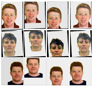 | |
| Fig. 6: | Successfully locating and defining the face in different translation positions, from left to right, respectively: left, up, down and right translations. Stirling University database (resized samples) |
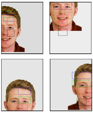 | |
| Fig. 7: | The failure in locating and defining the face in different severe translation positions, from left to right, respectively: left, up, down and right translations. Stirling University database (resized samples) |
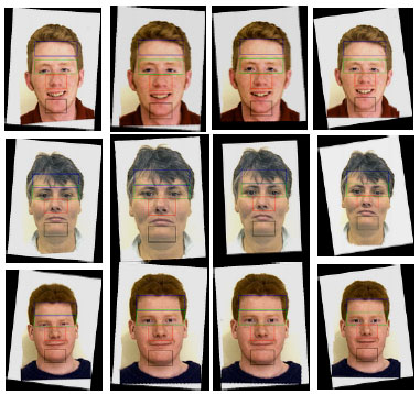 | |
| Fig. 8: | Successfully detecting and correcting rotations of -8, -4, +4, +8 degrees from right to left, respectively. Stirling University database (resized samples) |
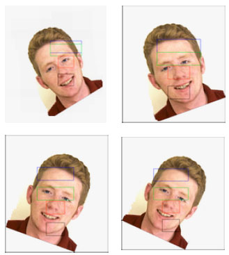 | |
| Fig. 9: | Failure in detecting and correcting rotations of -25, -20, +20, +25 degrees from right to left respectively. Stirling University database (resized samples) |
 | |
| Fig. 10: | Plot diagrams corresponding to the 69 feature vectors extracted from each pattern’s face image |
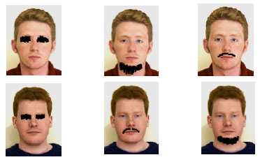 | |
| Fig. 11: | Modified face image to mimic facial details of sunglasses or facial hair. (resized samples) |
| Table 1: | Error rate of the system for different hidden layer neurons and patterns, case 1 |
 | |
| Table 2: | Error rate of the system for different hidden layer neurons and patterns case 2 |
 | |
From Table 2 systems performance degraded noticeably due to the vast variances in the extracted features when the facial details were added to the face images. In this case it`s very important to increase the number of hidden neurons and employ the cross validation technique during the training phase.
CONCLUSION
From the earlier results and since we couldn`t find any studies for recognizing colored faces for the same database which we experimented on and taking into account the large image sizes and the computational efficiency of this approach, we may conclude that our scheme performs fairly good under the stable conditions of lighting and scale.
Our system could be employed along with other sub-systems like speaker recognition, or finger print in a stand-alone Identity Verification system, in such a way that the total error is minimized and the overall system`s accuracy increased.
REFERENCES
- Brunelli, R. and T. Poggio, 1993. Face recognition: Features versus templates. IEEE Trans. Pattern Anal. Mach. Intell., 15: 1042-1052.
CrossRefDirect Link - Dai, Y. and Y. Nakano, 1998. Recognition of facial images with low resolution using a Hopfield memory model. Pattern Recog., 31: 159-167.
Direct Link - Daubechies, I., 1990. The wavelet transform, time-frequency localization and signal analysis. IEEE Trans. Inform. Theory, 36: 961-1005.
CrossRefDirect Link - Juell, P. and R. Marsh, 1996. A hierarchical neural network for human face detection. Pattern Recognit., 29: 781-787.
CrossRefDirect Link - Lawrence, S., C.L. Giles, A.C. Tsoi and A.D. Back, 1997. Face recognition: A convolutional neural-network approach. IEEE. Trans. Neural Networks, 8: 98-113.
CrossRefDirect Link - Lin, C.H. and J.L. Wu, 1999. Automatic facial feature extraction by genetic algorithms. IEEE Trans. Image Process., 8: 834-845.
CrossRef - Nakamura, O. S. Mathur and T. Minami, 1991. Identification of human faces based on isodensity maps. Pattern Recognit., 24: 263-272.
CrossRefDirect Link - Wu, C.J. and J. Huang, 1990. Human face profile recognition by computer. Pattern Recognit., 23: 255-259.
CrossRefDirect Link - Yuille, A.L., P.W. Hallinan and D.S. Cohen, 1992. Feature extraction from faces using deformable templates. Int. J. Comput. Vision, 8: 99-111.
CrossRefDirect Link