
T.K. Kar
Department of Mathematics, Bengal Engineering and Science University, Shibpur Howrah-711103, India
U.K. Pahar
Barisha High School, Barisha, Kolkata-700008, India
Journal of Fisheries and Aquatic Science
Year: 2007 | Volume: 2 | Issue: 3 | Page No.: 195-205


ABSTRACT
This research is devoted to the study of the dynamical behavior and harvesting problems of a prey-predator fishery, for which a protective patch is established for the prey species. Thresholds, equilibria and stabilities are determined for the system. The possibilities of existence of bionomic equilibrium is also discussed. The optimal harvesting policy is studied and the solution is derived in the equilibrium case by using Pontryagin`s maximal principle. Some numerical simulations are taken to illustrate the established results.
PDF Abstract XML References Citation
How to cite this article
T.K. Kar and U.K. Pahar, 2007. A Model for Prey-predator Fishery with Marine Reserve. Journal of Fisheries and Aquatic Science, 2: 195-205.
DOI: 10.3923/jfas.2007.195.205
URL: https://scialert.net/abstract/?doi=jfas.2007.195.205
DOI: 10.3923/jfas.2007.195.205
URL: https://scialert.net/abstract/?doi=jfas.2007.195.205
INTRODUCTION
This study analyzes the fishery management in the presence of an endangered predator that competes with humans for commercially viable prey. In the past, natural predators were implicit in the fishery model. We, however, explicitly model the predator-prey relationship given that endangered predators can be found in many fisheries and the importance of allowing these predator populations to expand in conjunction with maximizing rents in the fishery. Because traditional predator controls are not possible when the predator is endangered, we focus on harvesting effort controls over the prey’s habitat as a means to maintain the predator-prey relationship and sustain the economic viability of the fishery.
Brauer and Soudack (1979, 1981) and Myerscough et al. (1992) studied a general model of prey-predator interaction under constant harvesting or stocking and developed a comprehensive picture of the dynamics of the harvested model. Dai and Tang (1998) have given complete mathematical analysis of a prey-predator model with Holling Type I predator response (Holling, 1965), in which both the ecologically interacting species are harvested independently. In all these models the authors assumed constant catch. Azar et al. (1995) have made a comparative study between constant catch and constant harvesting effort in a prey-predator model and investigated a few significant phenomena such as a constant catch on the predator may destabilize a system that is stable when a constant harvesting effort is applied. Recently, Kar and Chaudhuri (2002) presented a mathematical model of nonselective harvesting in a prey-predator fishery. In their future work (Kar and Chaudhuri, 2003), they described the regulation of a prey-predator fishery by taxation as control instrument. Kar (2003) also presented a model to study the selective harvesting in a prey-predator fishery by introducing a time delay in the harvesting term.
Extensive and unregulated harvest of marine fishes can lead to the depletion of several fish species. One potential solution to these problems is the creation of marine reserves where fishing and other extractive activities are prohibited. Marine reserves not only protect species inside the reserve area but they can also increase fish abundance in adjacent areas. Marine reserves offer a promising alternative to fisheries management that normally relies on catch limits or restriction on gear and/or effort (Sutinen and Anderson, 1985). It is thought to enhance fisheries by protecting spawning stocks, providing refugia for pre-recruits and by exporting biomass to adjacent fishing grounds. It also have many non-fisheries benefits, such as protecting biodiversity and ecosystem structure, serving as biological reference areas and providing non-consumption recreational activities.
The analysis in this study consists of a prey-predator model in an aquatic habitat that consists of two zones: one free fishing zone and other is a reserve zone where fishing is not permitted. The choice of this model was motivated by the existence of Marine National Park, Kenya, a fully protected coral reef marine reserve comprising approximately 30% of former fishing ground and Marine National Park in the Iroise sea, a costal sea west of Brittany (France). Some recent works on exploitation of fishery resources with reserve area are Fan and Wang (2001), Dubey et al. (2003), Kar and Matsuda (2006), Sanchirico and Wilen (1999), Russ and Alcala (2004), Mangel (2000), Hanneson (1998) and Ami et al. (2005). This study is the modified model of Dubey et al. (2003) in the presence of a predator, which is seem to be more realistic. The objective of this study is to give a mathematical analysis for the dynamics of the species and to discuss the optimal harvesting policy.
THE MODEL AND PRELIMINARIES
If used properly and if drawn up in ways that involve and make biological sense for fishermen, protected areas may also become an effective tool in sustaining our fisheries by protecting key habitat and nursery areas.
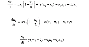
In this study, we consider the following predator-prey system in a two-patch environment:
 | (1) |
Here xi (t), (i = 1, 2) represents the prey population in the i-th patch, at time t≥0. We think of the patches with a barrier only as far as the prey population is concerned; the predator population has no barriers between patches. Thus y (t) stands for the total predator population for both patches. Patch 2 constitutes a reserve area for the prey and no fishing is permitted in this zone, while Patch 1 is an open-access fishery zone. We suppose that the prey migrate between two patches randomly. In the absence of predator, the growth rate of prey is assumed to be logistic. K and L are the carrying capacities; r and s are the intrinsic growth rates of prey species in the unreserved and reserved area, respectively. ε is a positive constant that can be viewed as the dispersal rate or inverse barrier strength. If ε = 0, then no member of the prey population can leave its patch. It is assumed that the net exchange from the j-th patch to the i-th patch is proportional to the difference xj - xi of population densities in each patch. γ and δ are predators death rate and intraspecific competition coefficients, respectively. E is the harvesting effort and q is the catchability coefficient.
Now it is easy to show that all solutions of system (1) are uniformly bounded.
Lemma 1: All the solutions of system (1) which start in R+3 are uniformly bounded.
Proof: We define the function
| (2) |
Therefore, the time derivative is found to be
For each μ > 0, upon computing the square separately in x and y the following inequality holds
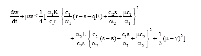 | (3) |
It is clear that the right hand side of inequality (3) is bounded for all (x1, x2, y) ∈ R+3, provided E is bounded. Thus we choose a V>0 such that
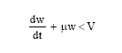 |
Applying the theory of differential inequalities developed by Birkhoff and Rota (1982), we obtain
| (4) |
which, upon letting ![]() Hence, all solutions of system (1) that start in R+3 are confined to the region B, where
Hence, all solutions of system (1) that start in R+3 are confined to the region B, where
![]()
EQUILIBRIA AND STABILITY ANALYSIS
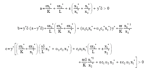
The possible steady states of (1) are P 0 (0, 0, 0), ![]() where
where
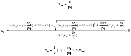
and P2 (x1*, x2*, y*) where
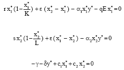 |
We shall now investigate the local behaviour of the model system (1) around the steady states.
For equilibrium point (0, 0, 0) the characteristic equation is
If , ![]() then P0 is a saddle point with stable manifold locally in the x1x2- plane and with unstable manifold locally in the y-direction.
then P0 is a saddle point with stable manifold locally in the x1x2- plane and with unstable manifold locally in the y-direction.
For the equilibrium point![]() , the characteristic equations is
, the characteristic equations is
 |
Therefore, P1 is a saddle point with a stable manifold locally in x1x2- plane and with unstable manifold locally in the y-direction.
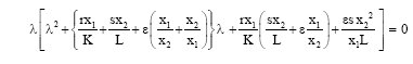
For the interior equilibrium point P2 (x1*, x2*, y*), the characteristic equation is
| (5) |
where
 |
By the Routh-Hurwitz criterion, it follows that all eigenvalues of (5) have negative real parts if and only if
a > 0, c > 0 and ab - c > 0
Here, a > 0, c > 0 and after a little algebraic manipulation it is easy to check that ab -c > 0
Hence, P2 (x1*, x2*, y*) is locally asymptotically stable.
From the point of view of ecological managers it may be desirable to have an equilibrium point which is globally asymptotically stable in order to plan harvesting strategy and keep sustainable ecological development.
So we shall discuss the global stability of the interior equilibrium point P2 (x1*, x2*, y*).
We make use of the standard Lyapunov function
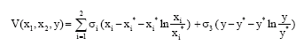 | (6) |
Its derivative along a solution of (1) takes the form
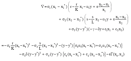 |
where
If we choose
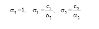 | (7) |
then we have,
Now it is easy to show that
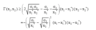 |
Thus we have
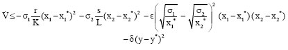 |
Clearly, if
 |
then for δ > 0 and ![]()
Hence, P2 is globally asymptotically stable.
Therefore, we have proved the following theorem.
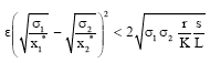
Theorem 1: The positive equilibrium point P2 (x1*, x2*, y*) is globally asymptotically stable if
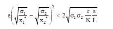 |
Simulation
For simulation let us take r = 3, s = 1.5, K = 50, L = 40, ε = 0.5, α1 = 0.2, α2 = 0.2, γ = 0.6, δ = 0.05, c1 = 0.03, c2 = 0.04, E = 2, q = 0.01 in appropriate units.
From the theory establishedearlier the interior equilibrium point P2 (19.5, 10.2, 7.86) is globally asymptotically stable.
From the Fig. 1, we may conclude that the steady state P2 is globally asymptotically stable. Hence the theory establishedearlier is verified.
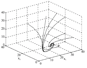 | |
| Fig. 1: | Phase space trajectories with reference to different initial levels |
BIONOMIC EQUILIBRIUM AND OPTIMAL HARVESTING POLICY
The bionomic equilibrium is said to be achieved when the total revenue is obtained by selling the harvested biomass equals the total cost utilized in harvesting it. Let c be the constant fishing cost per unit effort and p constant price per unit biomass of landed fish in the unreserved area. Then the economic rent (revenue at any time) is given by
| (8) |
Now if c > pqx1, i.e., if the fishing cost exceeds the revenue, then the economic rent obtained from the fishery becomes negative and the fishery will be closed. Hence, for the existence of bionomic equilibrium, it is natural to assume that c < pqx1.
The bionomic equilibrium (x1∞, x2∞, y∞, E∞) is the positive solutions of
Solving these equations we get,
 |
and
If E > E∞, then the total cost utilized in harvesting the fish population would exceed the total revenues obtained from the fishery. Hence some of the fishermen would be in loss and naturally they would withdraw their participation from the fishery. Hence E > E∞ cannot be maintained indefinitely. If E < E∞, then the fishery is more profitable and hence in an open access fishery it would attract more and more fishermen. This will have an increasing effort on the harvesting. Hence E < E∞ also cannot be maintained indefinitely.
Now our objective is to select a harvesting strategy that maximizes the present value
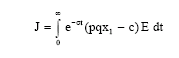 | (9) |
of a continuous time-stream of revenues. Here σ is the instantaneous annual discount rate. The problem (9), subject to the population Eq. 1 and control constants 0≤E≤Emax can be solved by applying Pontryagin's maximum principle (Pontryagin et al., 1964). Emax stands for a feasible upper limit on the harvesting effort.
The Hamiltonian for the problem is given by
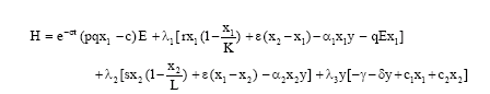 |
where λ1, λ2 and λ3 are adjoint variables and ![]() is called the switching function (Clark, 1990).
is called the switching function (Clark, 1990).
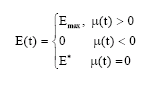
Since Hamiltonian H is linear in the control variable, the optimal control will be a combination of bang-bang controls and the singular control. The optimal control E(t) which maximizes H must satisfy the following conditions:
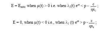
λ1(t) eσt is the usual shadow price (Clark, 1990) and p-is the net economic revenue on a unit harvest. This shows that E = Emax or 0 according as the shadow price is less than or greater than the net economic revenue on a unit harvest. Economically, the first condition implies that if the profit after passing all the expenses is positive, then it is beneficial to harvest up to the limit of available effort. Second condition implies that when the shadow price exceeds the fisherman's net economic revenue on a unit harvest, then the fisherman will not exert any effort.
When μ(t) = 0, i.e., when the shadow price equals the net economic revenue on a unit harvest, then the Hamiltonian H becomes independent of the control variable ![]() This is the necessary condition for the singular control E*(t) to be optimal over the control set 0 < E* < Emax.
This is the necessary condition for the singular control E*(t) to be optimal over the control set 0 < E* < Emax.
Thus the optimal harvesting policy is
 | (10) |
Again μ (t) = 0, implies that
| (11) |
This implies that the total user cost of harvest per unit effort must be equal to the discounted value of the future profit at the steady state effort level.
Now, the adjoint equations are
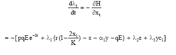 |
and
We seek to find optimal equilibrium solution of the problem so that x1, x2, y and E can be treated as constants. Therefore, adjoint equations become
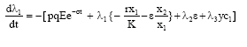 | (12) |
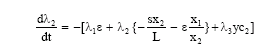 | (13) |
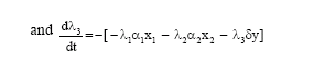 | (14) |
Now eliminating λ2 and λ3 from Eq. 12, 13 and 14 we get
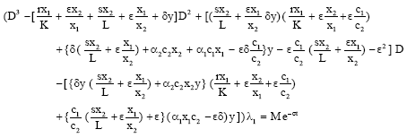 |
![]()
The auxiliary equation is
 |
Let its roots are m1, m2 and m3, then the general solution is
where
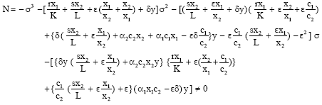 |
The shadow price eσt λ1(t) remains bounded as t → ∝ if and only if A1 = B1 = C1 = 0 and then![]()
Now substituting λ1 (t) in (11) we get
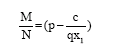 | (15) |
Equation 15, together with Eq.![]() gives the optimal equilibrium populations x1 = x1σ, x2 = x2σ and y = yσ.
gives the optimal equilibrium populations x1 = x1σ, x2 = x2σ and y = yσ.
When σ → ∝, Eq. 15 leads to the obvious result p q x1∞ = c, that implies
π (x1∞, x2∞, y∞, E) = 0
This shows that infinite discount rate leads to complete dissipation of economic revenue.
Using (15), we have
Since M is of O(σ) where N is O(σ2), we see that π is O(σ -1). Thus π is a decreasing function of σ (≥ 0). We, therefore, conclude that σ = 0 leads to maximization of π.
CONCLUDING REMARKS
The present study deals with a problem of harvesting in a prey-predator type fishery model with a reserve zone for prey species. Results on the local and global stability of the positive steady state are obtained. In order to have global stability, our criterion requires that the dispersal rate ε must be bounded above by some related constant. We then examine the possibilities of existence of bionomic (biological as well as economic) equilibria of the exploited system. Next, the optimal harvesting policy has been obtained using Pontryagin's maximum principle. We have discussed both bang-bang control and singular control. In the case of optimal equilibrium solution, it is found that the shadow prices remain constant over time in optimal equilibrium when they satisfy the transversality condition. Also the total user cost of harvest per unit effort equals the steady state effort level. It is proved that zero discounting leads to maximization of economic revenue and that an infinite discount rate leads to complete dissipation of economic rent.
ACKNOWLEDGMENT
The first author would like to thank Japan Society for the Promotion in Sciences (JSPS) for financially supporting the research (P05109).
REFERENCES
- Ami, D., P. Cartigny and A. Rapaport, 2005. Can marine protected areas enhance both economic and biological situations? Biologies, 328: 357-366.
CrossRefDirect Link - Azar, C., J. Holmberg and K. Lindgren, 1995. Stability analysis of harvesting in a predator-prey model. J. Theor. Biol., 174: 13-19.
Direct Link - Dai, G. and M. Tang, 1998. Co-existence region and global dynamics of a harvested predator prey system, SIAM. J. Applied Math., 58: 193-210.
Direct Link - Dubey, B., P. Chandra and P. Sinha, 2003. A model for fishery resource with reserve area. Nonlinear Anal. Real World Appl., 4: 625-637.
Direct Link - Fan, M. and K. Wang, 2001. Study on harvested population with diffusional migration. J. Syst. Sci. Comp., 14: 139-148.
Direct Link - Hanneson, R., 1998. Marine reserves: What would they accomplish? Mar. Resour. Econ., 13: 159-170.
Direct Link - Kar, T.K. and K.S. Chaudhuri, 2002. On nonselective harvesting of a multi-species fishery. Int. J. Math. Edu. Sci. Technol., 33: 543-556.
Direct Link - Kar, T.K., 2003. Selective harvesting in a prey-predator fishery with time delay. Math. Comp. Model., 38: 449-458.
Direct Link - Kar, T.K. and H. Matsuda, 2006. Modelling and analysis of marine reserve creation. J. Fish. Aquatic Sci., 1: 17-31.
CrossRefDirect Link - Mangel, M., 2000. On the fraction of habitat allocated to marine reserves. Ecol. Lett., 3: 15-22.
Direct Link - Myerscough, M.R., B.F. Gray, W.L. Hogorth and J. Norbury, 1992. An analysis of an ordinary differential equation model for a two- species prey-predator system with harvesting and stocking. J. Math. Biol., 30: 389-411.
Direct Link - Sanchirico, J.N. and J.E. Wilen, 1999. Bioeconomics of spatial exploitation in a patchy environment. J. Environ. Econ. Manage., 37: 129-150.
Direct Link