
Cihan Altuntas
Konya Technical University, Faculty of Engineering and Natural Science, 42075 Selcuklu Konya, Turkey
LiveDNA: 90.37081
Journal of Applied Sciences
Year: 2022 | Volume: 22 | Issue: 6 | Page No.: 329-341


ABSTRACT
Background and Objective: Image matching is a bottleneck that must be surpassed in photogrammetric measurement, camera calibration and computer vision. This study investigated the performances of the well-known feature point detectors in automatic matching. Materials and Methods: A large base-to-height ratio of stereo images creates perspective distortion and the selection of an object’s small shape properties from the image becomes difficult. Therefore, a large base-to-height ratio affects matching and measurement accuracy in photogrammetry. The relative variations on the scale of stereo images also make it difficult to create conjugate points between them. Different base-to-height and various scale stereo images were evaluated to compare the matching performance of these operators. Results: The results show that the number of matched feature points decreases when the base-to-height ratio of the images is increased. The SIFT, ASIFT and SURF operators did not match the images with a base-to-height ratio larger than 1.5 and a scale change of more than three times. Finally, ASIFT generated more matched points than SIFT and SURF. Conclusion: These findings are useful for automatic three-dimensional measurement from stereo images. Three-dimensional measurement can be performed with fewer images without any force on computer capacity. The imaging positions and point of view angles for multiview evaluations should also be planned according to the limitations of these operators.
PDF Abstract XML References Citation
Copyright: © 2022. This is an open access article distributed under the terms of the creative commons attribution License, which permits unrestricted use, distribution and reproduction in any medium, provided the original author and source are credited.
How to cite this article
Cihan Altuntas, 2022. Feature Point-Based Dense Image Matching Algorithm for 3-D Capture in Terrestrial Applications. Journal of Applied Sciences, 22: 329-341.
DOI: 10.3923/jas.2022.329.341
URL: https://scialert.net/abstract/?doi=jas.2022.329.341
DOI: 10.3923/jas.2022.329.341
URL: https://scialert.net/abstract/?doi=jas.2022.329.341
INTRODUCTION
Photogrammetric measurement has largely been automated thanks to developments in related disciplines. Many innovations in image processing and computer technology have been adapted to photogrammetric evaluation and automation has largely been practised in its current state. Automatic dense image matching is a major step in the historical development of photogrammetric evaluation. Dense image matching can be practised without knowledge of any technical information about the process. Nevertheless, technical details of the processes contribute to the efficient measurement and analysis of the results.
Image matching is essential to estimate the imaging geometry in stereophotogrammetry. The imaging geometry is created by intersecting homolog rays from the images via the epipolar constraint. Arbitrary aerial photogrammetric images have very similar perspectives and scales. Therefore, automatic image matching in aerial photogrammetry is not a complicated task and least-squares matching has been exploited to achieve precise image matching1,2. However, stereo images in close-range photogrammetry can be found at different scales, orientations and perspectives. The Scale Invariant Feature Transform (SIFT)3 algorithm has been extensively used to automatically match the close-range images in three-dimensional measurement, cultural heritage documentation, mobile measurement, object tracking, etc. Then, the Affine SIFT (ASIFT)4 and Speeded Up Robust Features (SURF)5 operators were introduced because they addressed the disadvantages of the SIFT algorithm such as its long computation time.
The SIFT operator created a new era in automation to match overlapping images3. The SIFT has been used for automatic image matching in photogrammetric measurement1,6, robot navigation7, feature tracking8 and camera calibration9. Many different versions of the SIFT have been introduced for faster and more efficient matching. The performance analysis of the SIFT in photogrammetric applications was conducted by Lingua et al.10. In addition, an auto-adaptive SIFT operator was validated using several aerial images acquired by an Unmanned Aerial Vehicle (UAV) system. The ASIFT has been developed to consider affine image deformations from the orientation and rotation of the images that have been comprised4. The SURF ignores some properties of images’ points of interest and it defines feature points in fewer dimensional spaces, unlike SIFT5. The SURF is extensively used for simultaneous localization and mapping applications due to its fast computation speed.
Image acquisition without detailed planning requires a denser set of viewpoints with larger overlaps to achieve the right coverage for reliable reconstruction. The image matching procedure forces the computer capacity and computational time to determine which pairs of images have tie points. A systematic survey for tie point generation from large unordered image collections was introduced in Hartmann et al.11. The technique relies on the parameterization of an image region and has been proven to be successful for matching by tackling issues such as scale, orientation or illumination changes. In addition, many studies show that image features learned and matched via deep learning outperform those of the previously described algorithms12,13. The ORB (Oriented FAST and Rotated BRIEF) binary descriptor is also constructed via machine learning. This descriptor maximizes the descriptor’s variance and minimizes the correlation under various orientation changes14.
Least squares matching does not significantly improve the matching accuracy of automatically generated tie points1,15. In addition, photogrammetric measurements with automatically or manually selected tie points have a close level of accuracy16.
The photogrammetric triangulation of a set of matched feature points constitutes a three-dimensional point cloud, which is called a sparse point cloud as inhomogeneous distribution. The number of matched feature points is essential for the relative orientation and translation of the images. The feature point operators constitute matched points as independent of the relative position and scale of the images. The studies in the literature have largely focused on image brightening and object-related achievements with matching operators, especially SIFT17. However, a stereo image could be recorded in different positions concerning the base-to-height ratio and relative scale in close range measurement. In this study, the feature point detection and matching performances of the well-known SIFT, ASIFT and SURF operators were investigated with various imaging configurations.
MATERIALS AND METHODS
Study area: The stereo images for matching were collected from the historical building in Konya, Turkey, in May, 2019.
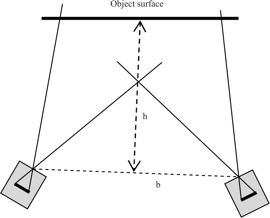
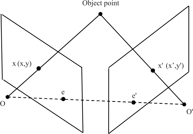
Imaging geometry: The overlapping images, also called stereo images are recorded from two stations. The distance between the image centres is the base (b) and the approximate distance from the base to the object is the imaging distance or height (h) given in Fig. 1.
 |
| Fig. 1: | Overlapping images geometry |
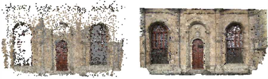 |
| Fig. 2: | Sparse (12587 points) and dense (680912 points) point cloud measurement data |
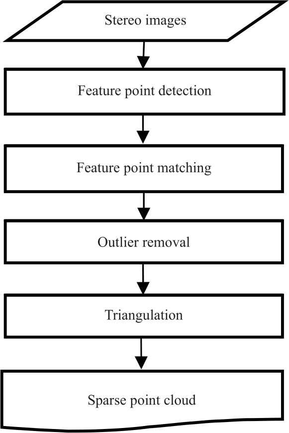 |
| Fig. 3: | Automatic stereo image matching and sparse point cloud generation pipeline |
A large base-to-height ratio creates perspective distortion and the selection of an object’s small shape properties from the image becomes difficult. Therefore, a large base-to-height ratio affects matching and measurement accuracy in photogrammetry. In addition, relative variations in the scale of stereo images also make it difficult to create conjugate points between the images.
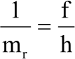
The image scale (mr) is estimated with the edge ratio of triangulations that have been formed on the side of the camera and object and is given as follows:
 | (1) |
where, f is the focal length and h is the average imaging distance between the base and object. According to Eq. 1, when the imaging distance is increased, the image scale will be decreased.
An image pixel represents the overflow property of its corresponding patch on the object's surface. Many small patch properties on a pixel projection area are not represented in the image. Hence, a large-scale image has more details than a small-scale image. The relationship between the pixel dimensions and the image scale (mr) is expressed as:
GSD = p.mr | (2) |
where, GSD is the ground sampled distance of one-pixel projection and p is the pixel dimension on the camera sensor. If the image scale increases, small object details become selectable. Therefore, large variations between the image scales affect the number of matched points for automatic matching.
Automatic image matching: Automatic image matching constitutes corresponding points by matching similar feature points from the images. After removing the outlier matches, three-dimensional coordinates are estimated for the rest of the matched feature points using photogrammetry principles. These object coordinates constitute the sparse point cloud that has nonuniform point spaces. More conjugate points are then generated with the estimated exterior image parameters to generate dense point clouds that have uniform point spaces as shown in Fig. 2.
Automatic image matching and point cloud creation procedures are collectively called the structure-from-motion algorithm18. The algorithm in Fig. 3 can also be realized without camera calibration parameters. Commercial photogrammetry software allows users to restrict the number of detected and matched feature points. In this way, multi-image matching does not force the computer capacity.
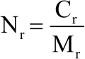
The achievements of feature point operators for image matching are evaluated with the number of matched feature points (Mr) and correct matched feature points (Cr).
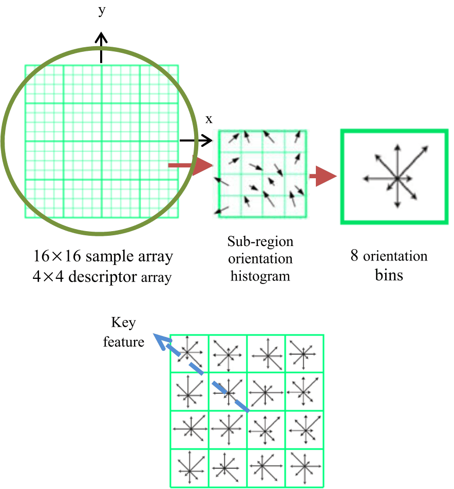 |
| Fig. 4: | Feature point summarizing the orientation and rotation contents over 4×4 sub-regions Every feature point is described with a length of 128 vectors representing a 4×4 array with 8 orientation bins |
 |
| Fig. 5: | ASIFT related Affine perspective image deformations and their geometric description |
Then, the correct match ratio (Nr) is estimated as below:
 | (3) |
SIFT operator: A feature point operator detects image points that are stable despite changes to the scale, orientation, brightness and perspective of the image. The SIFT operator describes the points of interest with a 128-dimensional feature vector3. The operator extracts feature points as the maximum response of the Difference of Gaussians (DoG) function. Feature points are detected in the DoG scale space as the local maxima and minima of D(x, y, σ) and expressed as:
D(x, y, σ) = L (x, y, kσ)-L (x, y, σ) | (4) |
L(x, y, σ) = G (x, y, σ)×I (x, y) | (5) |
where, k is the constant multiplicative factor, L(x, y, σ) defines the scale-space with the Gaussian kernel G(x, y, σ) and I(x, y) is the input image (Eq. 5).
At a given image scale, each image point is compared to eight adjacent pixels and nine neighbours in the scales above and below to detect the local maxima and minima of the DoG scale space. The local maxima and minima are then classified as feature points. To select stable feature points, the local extreme values of D(x, y, σ) must be higher than a certain threshold. The DoG scale space ensures that the feature points are invariant to scale changes but sensitive to rotation. To avoid these problems during feature matching operations as shown in Fig. 4, the SIFT detector assigns a canonical orientation to each feature point based on the local radiometric properties of the neighbouring pixels3,10.
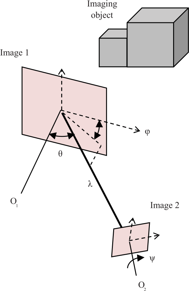
ASIFT operator: The ASIFT operator considers affine image deformations composed of orientations and rotations of the images to define the feature points. Thus, ASIFT covers all six parameters of the affine transform. The ASIFT represents image perspective distortions that are composed of different point of view angles. The ASIFT can successfully detect match points from corresponding images, even when they have high affine distortions. The ASIFT creates many sample simulations to obtain imaging views of the initial two images. As given in Fig. 5, the sample view simulations are obtained by varying the scale (λ) and orientation parameters, which are called the longitude (φ) and latitude (θ) angles. Camera rotation around its optical axis is defined as the camera spin parameter (ψ). The ASIFT is performed in the three steps described below4.
Each image is transformed by simulating all possible longitude (φ) and latitude (θ) angles of the optical axes of the two cameras. The tilt parameter is related to the rotation angle latitude as t = 1/|cosθ|. If two images have similar camera positions, t is 1. These rotations and tilts are performed with a few latitude and longitude angles until the simulated images stay close to each other
| • | The simulated images are matched using SIFT or other image matching methods |
| • | Epipolar geometry is applied using the optimized random sampling algorithm method19 to eliminate possible false matches |
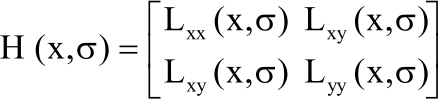
SURF operator: The SURF relies on the scale-space representation based on the Hessian matrix, which lends itself to the use of integral images20 to drastically reduce the computational time. Given a point x = (x, y) in an image, the Hessian matrix H (x, σ) in x at scale σ is defined as:
 | (6) |
where, Lxx (x, σ), Lxy (x, σ) and Lyy (x, σ) are the convolutions of the Gaussian second-order derivative with the image at point x.
The method includes two basic steps. First, the Haar wavelet responses in the x and y directions are estimated in a circular neighbourhood around the point of interest of integral images. The integral images ensure the operator’s speed. Then, the wavelet responses are converted to a vector with two strengths represented in the horizontal and vertical directions. The summed orientation is then estimated by calculating the sum of all horizontal and vertical responses within the orientation window. The point of interest is oriented to the longest vector. Second, the detected point of interest is described using a squared window that has a summed vector orientation5.
The SURF ignores some properties of the feature points and defines 64-dimensional feature vectors, which is distinct from SIFT. In this way, it detects and matches feature points faster than the other operators and it has been extensively utilized in simultaneous localization and mapping applications. The SURF feature points can also be defined by 128-dimensional feature vectors for further applications.
Feature point matching: Once feature points are detected from two images, possible match points can be found automatically. A feature vector in one of the images is matched with a similar high-level feature vector in the other image without using any exterior camera parameters. Finding candidate matching descriptor points between the overlapped images is typically performed using the Euclidean distance or kD-tree approach. The kD-tree is a quick method to search for matching candidates1. The kD-tree search performance is increased by using principal component analysis21. Artificial neural network techniques also improve the process of finding the candidate matching points from kD-tree search structures. Low precision and a speed-up of three orders of magnitude for an exhaustive linear search can be achieved through an artificial neural network11,22. Best bin fast, which is a variant of the kD tree search algorithm, makes indexing in higher dimensional spaces practical23.
The Euclidean distance is widely used to compare the similarities of feature vectors. The constraint described by Lowe3 can be used to screen candidates. It estimates the Euclidean distances between candidate feature points. A constraint between the first-and the second-best candidates are added to make the results even more distinctive. To find the possible feature points in the other image, all distances are sorted from shortest to longest. If the ratio from a minimum distance to the next minimum distance is lower than a certain threshold (t), the pair of feature points is selected as a candidate match, otherwise, the pair is discarded. The standard value of t is 0.6. However, lower or higher thresholds are possible. A low threshold leads to highly reliable matched feature points and a high threshold leads to a high number of matched points with relatively low reliability24.
Outlier removal: The matched feature points have a few outliers that cannot be detected with the proposed matching strategy. Deep learning classifiers can be used to determine the correctness of an arbitrary putative match. The classifier is trained based on a general match representation associated with each putative match. The learned classifier can determine the correctness of an arbitrary putative match within linearithmic time complexity25.
The epipolar constraint is usually applied to remove the outliers from a set of matched points. This constraint requires the corresponding image and object points to be on the same plane. The epipolar constraint is checked using a subset of the matched feature points. The subset points can be selected using the random sample consensus (RANSAC)26, least median of squares (LMS)27 or maximum a posteriori sample consensus (MAPSAC)28 methods. The RANSAC algorithm has usually been adopted to remove outlier matched feature points29-31. The number of subset points should be more than the probability ratio of an incorrect match.
 |
| Fig. 6: | Epipolar geometry |
The epipolar constraint can be realized by the essential (E) matrix when the intrinsic parameters of the cameras are known and the fundamental (F) matrix otherwise32,33. The F matrix, covering the internal and external camera parameters, is an arithmetic definition of epipolar geometry. Once a set of corresponding image coordinates between two views is given as x = [x, y, 1]T and x' = [x', y', 1]T, the epipolar constraint is given as:
xT = Fx' = 0 | (7) |
Each point match gives one linear equation in the unknown entries of F. Specifically, a linear equation corresponding to a match point (x, y, 1) and (x', y', 1) is written as:
x'xf11+x'yf12+x'f13+y'xf21+y'yf22+y'f23+xf31+yf32+f33 = 0 | (8) |
From a set of n point matches, we obtain a set of linear equations of the form as:
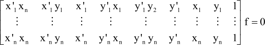 | (9) |
when, F33 = 1, the eight-point algorithm is applied to compute the F matrix32.
The F matrix represents a connection between a point in the first image and the epipolar line in the second image. In Fig. 6, once a point on the first image is transformed into the other image, it must be on the epipolar line. Correct match points such as x (xi, yi, 1) and x' (x'i, y'i, 1) minimize the epipolar constraint exactly.
Possible match points![]() can be found by minimization of the cost function, given as:
can be found by minimization of the cost function, given as:
 | (10) |
where, d is the Euclidean distance between the transferred and known position of a point. This is equivalent to minimizing the reprojection error for a pointthat is mapped to and by F. The cost function could be minimized using a numerical minimization method. A close approximation to the minimum may also be found using Sampson error which has a threshold (t) to determine if it is an outlier match32. An initial value of 5 pixels is usually set as the threshold32,34.
The F matrix is estimated using randomly selected corresponding points on the subset. d is calculated for each putative correspondence. The number of inliers consistent with F is estimated with satisfying the condition d<t. This process is repeated for each sample of match points until the solution with most inliers is retained. The F matrix, which has more inlier matched points, is then accepted as correct and is used to select outlier matches.
Base to height ratio related matching: The overlapping images with varying base-to-height ratios were taken from a historical structure with a Nikon P50 camera (f = 4.521 mm). Fig. 7a-e shows the images that were automatically matched using the feature point detectors (www.ipol.im/). The epipolar geometry was applied using the F matrix, which was estimated from the subset points selected by RANSAC. The elimination criterion was identified by applying Eq. 7 as one pixel for outlier removal. The matching results of the feature points are given in Table 1. According to Table 1, if the base-to-height ratio (b/h) increased, the number of matched points decreases. When the ratio exceeds 1.5, all three operators failed to generate the conjugate points. On the other hand as expected, Cr of SIFT for b/h level of 0.38 is 706 and 962 for t = 0.6 and t = 0.8, respectively. However, their Nr is 91.10 and 84.38%, respectively. Table 1 also shows that the Nr of ASIFT is higher than the other operators because it takes into account affine parameters to match the feature points. The Nr of ASIFT is 98.95 and 91.67% for b/h of 0.38 and 1.50, respectively. However, Nr of SIFT is 91.10 and 63.01% for b/h of 0.38 and 1.50, respectively. And Nr of SURF is 89.51 and 22.92% for b/h of 0.38 and 1.50, respectively. Figure 8a shows that the Cr of SIFT decreased when base/height ratios are increased. The Cr of SIFT is lower than the SURF and ASIFT. Figure 8b shows that the Nr of ASIFT has a stable level for all base/height ratios. However, the Nr of SIFT and SURF has been decreased by the base/height ratios increased. Image scale related matching: The matching results of the images which have different imaging distances and similar perspectives to the object are shown in Fig. 9a-f. The images in Fig. 9a have less difference (mr1/mr2 = 1.23) between the image scales, thus they have more matching. However, the image scales have the biggest difference (mr1/mr2 = 3.54) and thus fewer matching. The close-range images cover a smaller area than those taken from a longer distance. The main problem with matching large- and small-scale images is the selection of the same object points from the images that have different levels of detail. The performances of these three operators were evaluated by matching the images which have different scales. The overall matching results were provided in Table 2. The results show that the Mr decreased when the scale ratio (mr1/mr2) between the images increased. When the scale ratio reached 3.54 times, the SIFT was only able to create conjugate points. Table 2 also shows that the Cr is decreased by the scale ratio increased for all three operators. For example, Cr of SIFT is 843 and 36 for scale ratio (mr1/mr2) of 1.23 and 3.54, respectively. Nr of ASIFT is higher than the other operators because it takes into account affine parameters to match the feature points. The Nr of ASIFT is 99.96 and 96.23% for scale ratios of 1.23 and 3.08, respectively. However, Nr of SIFT is 78.63 and 18.89% and Nr of SURF is 85.73 and 41.24% for the scale ratio of 1.23 and 3.08, respectively. Figure10a shows that the Cr is decreased by the scale ratio (mr1/mr2) increased for all three operators. The Cr of SIFT is lower than the SURF and ASIFT. Figure 10b shows the Nr of ASIFT has a stable level for all scale ratios between the images. However, the Nr of SIFT and SURF is decreased by the scale ratios increased. Image scale and orientation related matching: The images in close range measurement are typically inconveniently positioned with each other in terms of scale and point of view angle. The abilities of the SIFT, ASIFT and SURF feature point operators to match the images that have different scales and point of view angles were tested in Fig. 11. The images were taken from distances of 8 m (mr1 = 1769) and 17 m (mr2 = 3804) away from the object. The intersection angle of their optical axis is 49 degrees. The matching results are given in Table 3. According to Table 3, the perspective and scale change between the stereo images decrease the match points and also the success of the operators. The SIFT is the most successful operator concerning Cr, which is 72. However, the Nr of ASIFT is higher than the SIFT and SURF and is 87.84. Object related matching: The automatic matching achievements of the feature point operators were evaluated for different surface properties of the object. The overlapping images were collected from the avenue, building, dam, historical heritage, rock surface and stone building. The avenue images are large plants and asphalt roads. The dome images include water surfaces that make it difficult to select any feature points. The building images have repeated patterns of windows. The image pairs given in Fig. 12 were automatically matched using the operators. Table 4 shows that the ASIFT operator acquired a larger Mr than the others for all the image sets. In addition, the Nr of ASIFT is larger than the SIFT and SURF for all cover types. It is a minimum of 90.35% for stone buildings. The SURF is more successful for the images which have repeated patterns such as windows of building in Fig. 12. The Nr of SURF is higher than the SIFT and is 52.92%. Reprojection error: After matching feature points from two or more overlapping images, the three-dimensional coordinates are computed using the camera's internal and external parameters and the image coordinates of the feature points. The object coordinates are simultaneously estimated for all the matched points by using bundle adjustment. When the object coordinates are reprojected on the images using the estimated camera parameters, the distance between a marked and reprojected point on the image is called a reprojection error. The reprojection error provides information regarding image orientation accuracy related to the matching. The results show that the low base-to-height ratio has a small reprojection error which means high accuracy matching. Figure 13a shows that a high base-to-height ratio makes reprojection errors larger. The reprojection error is increasing proportionally with the differences in the scale between the images as shown in Fig. 13b. The results show that the SIFT, ASIFT and SURF are unsuccessful in automatic image matching when the base-to-height ratio exceeds 1.5. However, SIFT and SURF can match images with a base-to-height ratio of 1.88. Nevertheless, the matching accuracy was not checked because the number of matched points was insufficient for estimating the F matrix. The number of correctly matched SIFT points is lower than those for ASIFT and SURF in these experiments. Regarding the correct match ratio, SURF had a lower ratio than the other methods as given in Table 1. The SURF is more successful in matching the images of repeated details. Table 4 shows the achievement of SURF to match the repeated patterns, such as reported in the literature5. For all the operators, when the base-to-height ratio is increased, the number of matched points decreases. Furthermore, SIFT exhibited outstanding results compared to ASIFT and SURF for matching scale-change images. The SIFT can match the images even if the scale ratio between the images is 3.54, while the other methods can only match the images that have a threefold scale change. ASIFT has a higher correct match ratio than the other methods. This achievement is related to the affine deformation that is considered in feature point detection in Table 2. As similar to the results given on the literature4, ASIFT has a high correct match rate for overlapping images of varying scale and perspective given in Table 3. A high threshold (t) used to find possible match candidates causes more outlier matches, as shown in Table 1 by matching the SIFT feature points for t=0.6 and t=0.8. Fathi and Brilakis30 and Barazzetti et al.1 also reported high matching for high threshold (t), but low correct match ratio. Fig. 10 shows that the number of matched points subsided for all operators when the scale change between the images was increased. The ASIFT has a higher correct match ratio than SIFT and SURF because it considers affine deformations, which are derived from the orientation and translation between the images. The SIFT and ASIFT operators define points of interest with 128-dimensional feature vectors. The SURF creates a 64-dimensional feature vector, thus, it is quick and often preferred for mobile measurement35. However, because the SURF feature vector has fewer properties for the interest points, it has more outlier matched points than the other operators. The RANSAC algorithm was proposed to increase the probability of correct matching points being sampled36. The SURF feature vector can be extended to 128 dimensions to overcome this weakness. Photogrammetry requires a base-to-height ratio of approximately 1 for stereo images for a highly accurate measurement. This should be considered when generating a point cloud from stereo images. The given matching limits may vary slightly for different image sets. Least squares matching increases the matching accuracy of the detected feature points. However, it makes a slight contribution to increasing measurement accuracy because the operators create many corresponding points through automatic matching. Moreover, least-squares matching is unsuccessful in stereo pairs with a scale variation of more than 30% and a crossing angle greater than 25 degrees1. The estimated large reprojection error for the high base-to-height ratio is compatible with the literature1,10. The studies performed report high matching for small base-to-height. Multi-image photogrammetric evaluation using a bundle adjustment can also be applied to attain highly accurate measurements considering the limits of these image matching operators. The image matching execution time is largely dependent on computer capacity. The time may vary depending on the resolution of the image but not cover content. This study provides practical guidelines for the strengths and weaknesses of the SIFT, ASIFT and SURF operators in the matching of overlapping images that have scale and point of view angle variations. The experiments were conducted using images of cultural heritage, which is an extensive application area of close-range photogrammetry with the aim of three-dimensional documentation. The results indicate that the imaging has to be done under particular geometric conditions for automated image matching. The base-to-height and scale ratio limits between the images are 1.50 and 3.08 for all three operators, respectively. The matching accuracy rate of ASIFT has higher than the SIFT and SURF and stable to change of perspective and scale between the images. These limits may vary slightly depending on the field of view coverage. The SURF is more successful in matching the images of repeated details. If the images are taken according to the achievements of these operators, three-dimensional measurement can be performed with fewer images without any force on computer capacity. Moreover, the imaging positions and point of view angles for multiview evaluations should be planned according to the limitations of these operators for efficient three-dimensional modelling. This study discovered the performances of the well-known feature point detectors in automatic matching. Three-dimensional measurements were performed with fewer images. The imaging positions of view angles for multiview evaluations also be planned.RESULTS
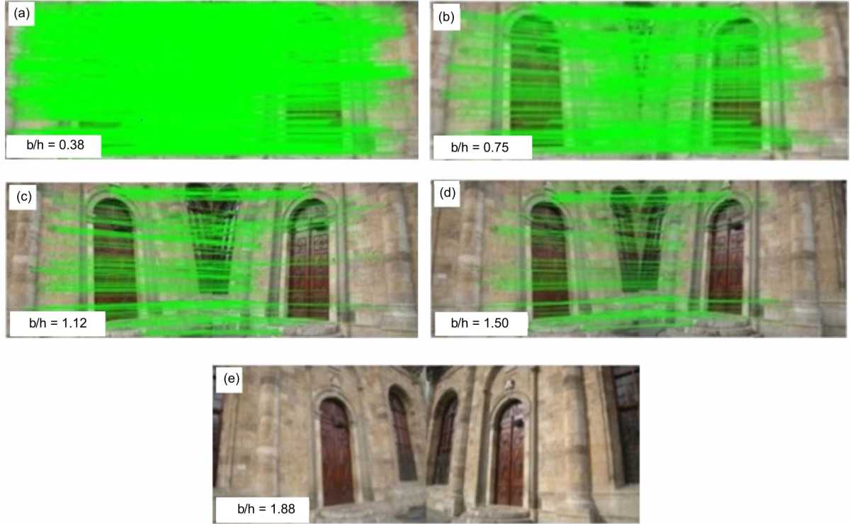
Fig. 7(a-e): Different base to height ratio overlapping images and SIFT matching results (t = 0.6)
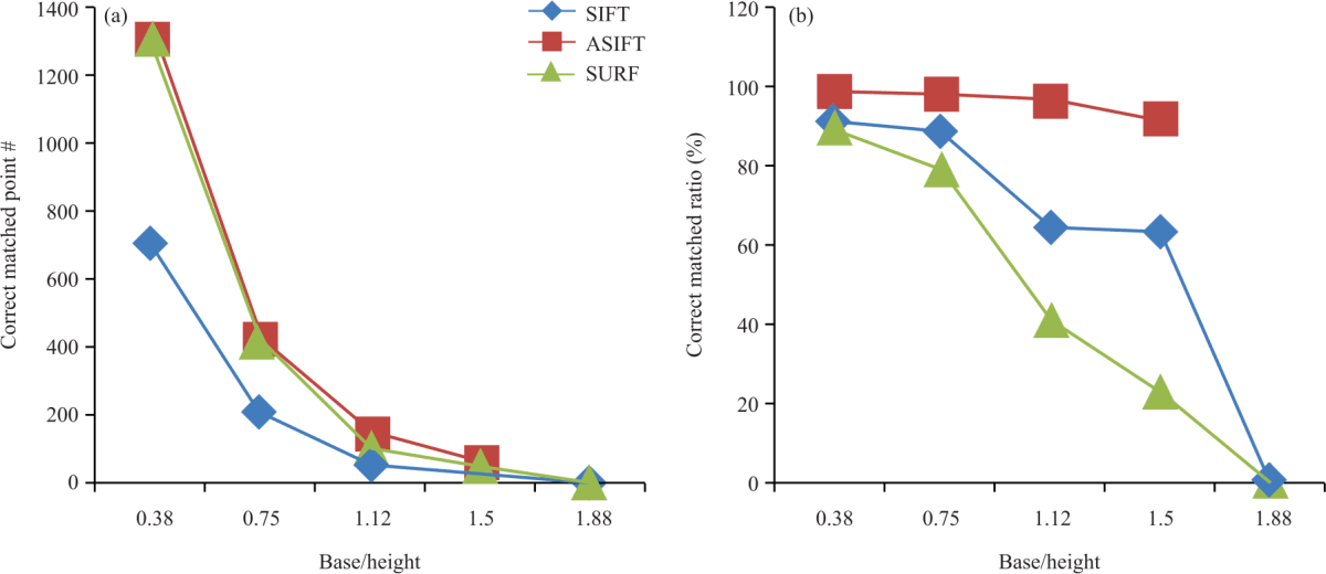
Fig. 8(a-b): Matching results of the different base to height ratio images, (a) Correct matched point and (b) Correct matched ratio
Table 1: Base to height ratio related matching (2048×1536 pixel array)
b/h (h = 6.40 m) OperatorstMatched points# MrCorrect match# CrCorrect match ratio Nr (%) 0.38 SIFT0.677570691.1 0.8114096284.38 ASIFT0.61329131598.95 SURF0.61459130689.51 0.75 SIFT0.623320688.41 0.860439164.74 ASIFT0.642842098.13 SURF0.652341479.16 1.12 SIFT0.6936064.52 0.846716936.19 ASIFT0.615314896.73 SURF0.625910640.93 1.5 SIFT0.6734663.01 0.840210425.87 ASIFT0.6726691.67 SURF0.61924422.92 1.88 SIFT0.63200 0.836100 ASIFT0.6000 SURF0.612500
Table 2: Image scale related matching (f = 4.521 mm, h1 = 5.20 m, mr1 = 1150)
Scale ratio mr1/mr2 OperatorsMatch point# MrCorrect match# CrCorrect match ratio Nr (%) 1.23 SIFT107284378.63 ASIFT2245224499.96 SURF2313198385.73 1.69 SIFT52232562.26 ASIFT53453399.81 SURF104879776.05 2.15 SIFT48225561.2 ASIFT46846699.57 SURF54536166.24 2.62 SIFT31410031.85 ASIFT11711598.29 SURF38422057.29 3.08 SIFT2865418.89 ASIFT535196.23 SURF29112041.24 3.54 SIFT2543614.17 ASIFT000 SURF20100
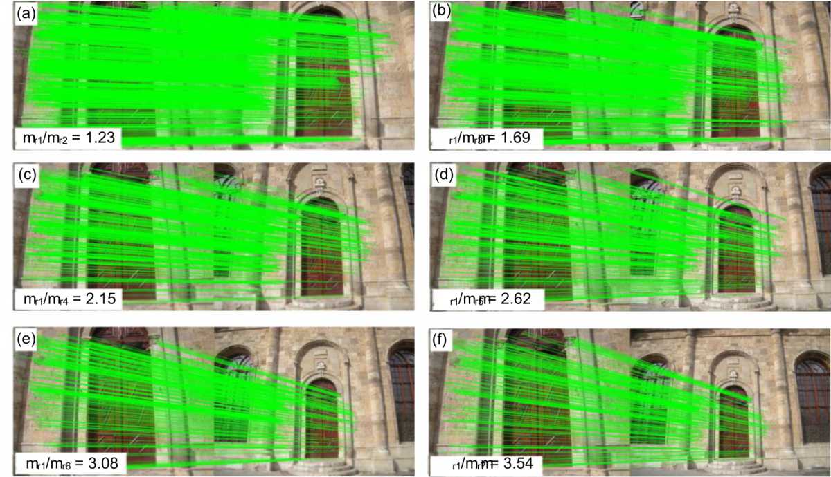
Fig. 9(a-f): Different scale image matching by SIFT detected feature points (mr1 = 1150)
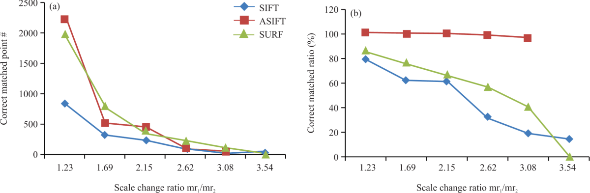
Fig. 10(a-b): Matching results for scale variations between the images, (a) Correct matched point and (b) Correct matched ratio
Table 3: Scale and orientation related matching
Image 1 feature points # (mr = 1769)Image 2 feature points # mr = 3804Match points # MrCorrect match # CrCorrect match ratio Nr (%) SIFT 284945514237217.02 ASIFT 1991131019746587.84 SURF 850785091444027.78
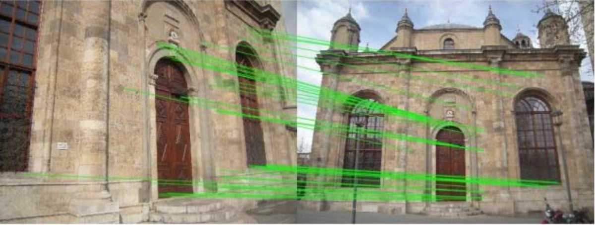
Fig. 11: Automatic matching results of the images that have a different scale and point of view angles (SIFT)
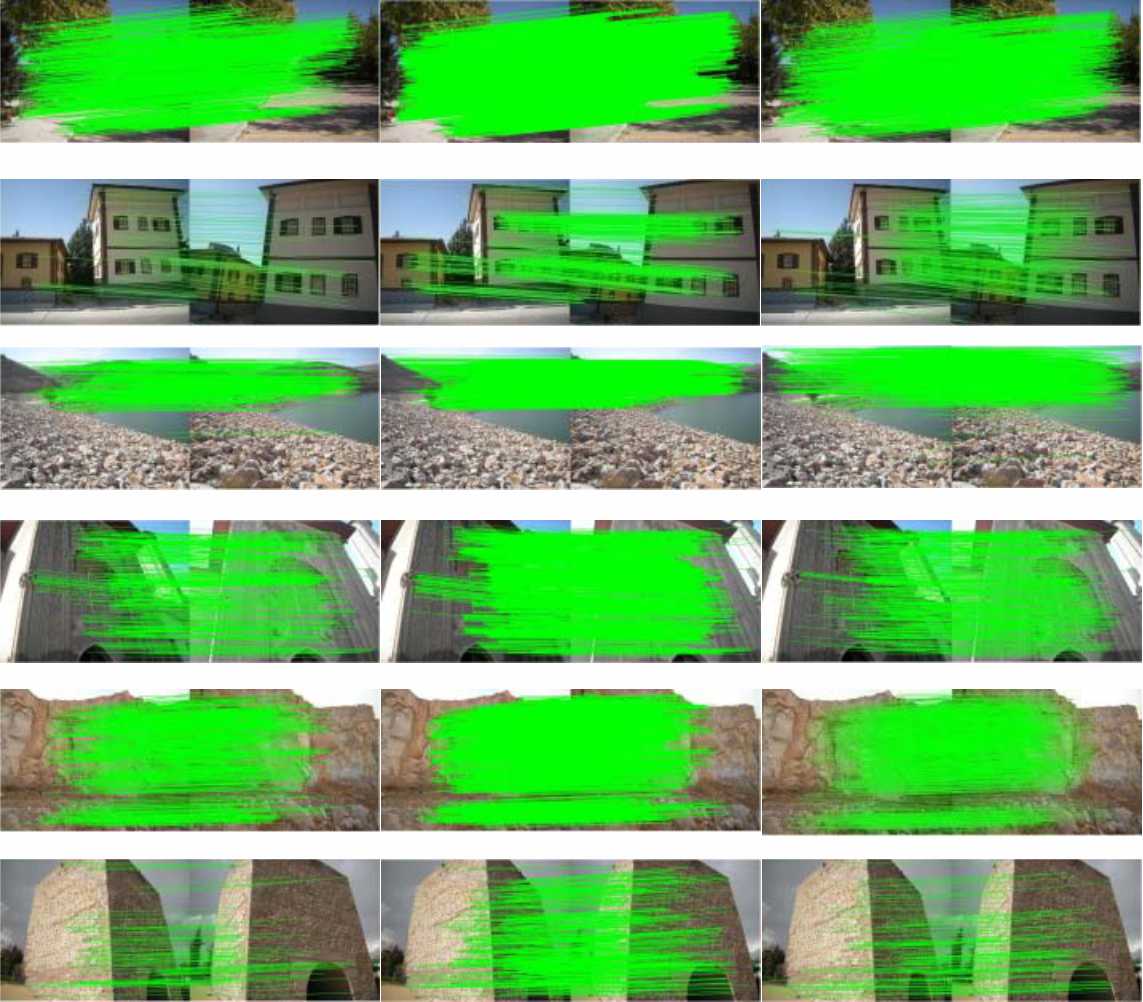
Fig. 12: Image matching results for different surface properties (t = 0.6)
Left to right SIFT, ASIFT and SURF
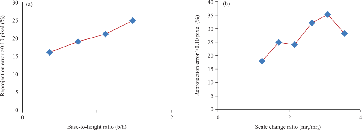
Fig. 13(a-b): Relationship between reprojection error and imaging geometry, (a) Base-to-height ratio makes reprojection errors and (b) Scale change ratio makes reprojection errors
Table 4: Image matching results for various cover of surfaces
Image object Metric SIFTASIFTSURF Avenue Feature 1#/ 2672342185705 Feature 2# 2453298125743 Mr 121260491638 Cr 112258021475 Nr (%) 92.5795.9290.05 Building Feature 1# 1787169665025 Feature 2# 1475123505002 Mr 134427359 Cr 51397190 Nr (%) 38.0692.9752.92 Dam Feature 1# 3126408676076 Feature 2# 3006392785967 Mr 3671485870 Cr 3411450737 Nr (%) 92.9297.6484.71 Historical heritage Feature 1# 1207133605463 Feature 2# 1380139935747 Mr 3231218527 Cr 2891148391 Nr (%) 89.4794.2574.19 Rock Feature 1# 2553261035920 Feature 2# 2602258015973 Mr 6512320753 Cr 5952230648 Nr (%) 91.496.1286.06 Stone building Feature 1# 1987260395686 Feature 2# 1575207675685 Mr 133570225 Cr 87515135 Nr (%) 65.4190.3560.00DISCUSSION
CONCLUSION
SIGNIFICANCE STATEMENT
REFERENCES
- Barazzetti, L., M. Scaioni and F. Remondino, 2010. Orientation and 3D modelling from markerless terrestrial images: Combining accuracy with automation. Photogramm. Rec., 25: 356-381.
CrossRefDirect Link - Bethmann, F. and T. Luhmann, 2011. Least-squares matching with advanced geometric transformation models. Photogrammetrie Fernerkundung Geoinf., 2011: 57-69.
CrossRefDirect Link - Lowe, D.G., 2004. Distinctive image features from scale-invariant keypoints. Int. J. Comput. Vision, 60: 91-110.
CrossRefDirect Link - Yu, G. and J.M. Morel, 2011. ASIFT: An algorithm for fully affine invariant comparison. Image Process. Line, 1: 11-38.
CrossRefDirect Link - Bay, H., A. Ess, T. Tuytelaars and L. van Gool, 2008. Speeded-Up Robust Features (SURF). Comput. Vision Image Understand., 110: 346-359.
CrossRefDirect Link - Karagiannis, G., F.A. Castro and D. Mioc, 2016. Automated photogrammetric image matching with SIFT algorithm and delaunay triangulation. ISPRS Ann. Photogramm. Remote Sens. Spatial Inf. Sci., III-2: 23-28.
CrossRefDirect Link - Li, X., X. Li, M.O. Khyam, C. Luo and Y. Tan, 2017. Visual navigation method for indoor mobile robot based on extended BoW model. CAAI Trans. Intell. Technol., 2: 142-147.
CrossRefDirect Link - Jin, R. and J. Kim, 2017. Tracking feature extraction techniques with improved SIFT for video identification. Multimedia Tools Appl., 76: 5927-5936.
CrossRefDirect Link - Li, C., P. Lu and L. Ma, 2010. A camera on-line recalibration framework using SIFT. Visual Comput., 26: 227-240.
CrossRefDirect Link - Lingua, A., D. Marenchino and F. Nex, 2009. Performance analysis of the SIFT operator for automatic feature extraction and matching in photogrammetric applications. Sensors, 9: 3745-3766.
CrossRefDirect Link - Hartmann, W., M. Havlena and K. Schindler, 2016. Recent developments in large-scale tie-point matching. ISPRS J. Photogramm. Remote Sens., 115: 47-62.
CrossRefDirect Link - Guo, Q., J. Xiao and X. Hu, 2018. New keypoint matching method using local convolutional features for power transmission line icing monitoring. Sensors, Vol. 18.
CrossRefDirect Link - Ma, J., X. Jiang, A. Fan, J. Jiang and J. Yan, 2021. Image matching from handcrafted to deep features: A survey. Int. J. Comput. Vision, 129: 23-79.
CrossRefDirect Link - Heinly, J., E. Dunn and J.M. Frahm, 2012. Comparative Evaluation of Binary Features. In: Computer Vision-ECCV 2012, Fitzgibbon, A., S. Lazebnik, P. Perona, Y. Sato and C. Schmid (Eds.), Springer, Berlin, Heidelberg, pp: 759-773.
CrossRefDirect Link - Giang, N.T., J.M. Muller, E. Rupnik, C. Thom and M. Pierrot-Deseilligny, 2018. Second iteration of photogrammetric processing to refine image orientation with improved tie-points. Sensors, Vol. 18.
CrossRefDirect Link - Mousavi, V., M. Varshosaz and F. Remondino, 2021. Using information content to select keypoints for UAV image matching. Remote Sens., Vol. 13.
CrossRefDirect Link - Chen, S., X. Yuan, W. Yuan, J. Niu, F. Xu and Y. Zhang, 2018. Matching multi-sensor remote sensing images via an affinity tensor. Remote Sens., Vol. 10.
CrossRefDirect Link - Granshaw, S.I., 2018. Structure from motion: Origins and originality. Photogramm. Rec., 33: 6-10.
CrossRefDirect Link - Moisan, L. and B. Stival, 2004. A probabilistic criterion to detect rigid point matches between two images and estimate the fundamental matrix. Int. J. Comput. Vision, 57: 201-218.
CrossRefDirect Link - Ehsan, S., A.F. Clark, N.U. Rehman and K.D. McDonald-Maier, 2015. Integral Images: Efficient algorithms for their computation and storage in resource-constrained embedded vision systems. Sensors, 15: 16804-16830.
CrossRefDirect Link - Huang, y., Z. Zhao, C. Qi, Z. Nie and Q.H. Liu, 2018. Fast point-based KD-tree construction method for hybrid high frequency method in electromagnetic scattering. IEEE Access, 6: 38348-38355.
CrossRefDirect Link - Chen, L., F. Rottensteiner and C. Heipke, 2021. Feature detection and description for image matching: From hand-crafted design to deep learning. Geo-Spatial Inf. Sci., 24: 58-74.
CrossRefDirect Link - Li, W., Y. Zhang, Y. Sun, W. Wang, M. Li, W. Zhang and X. Lin, 2020. Approximate nearest neighbor search on high dimensional data-experiments, analyses, and improvement. IEEE Trans. Knowl. Data Eng., 32: 1475-1488.
CrossRefDirect Link - Zhuo, X., T. Koch, F. Kurz, F. Fraundorfer and P. Reinartz, 2017. Automatic UAV image geo-registration by matching UAV images to georeferenced image data. Remote Sens., Vol. 9.
CrossRefDirect Link - Ma, J., X. Jiang, J. Jiang, J. Zhao and X. Guo, 2019. LMR: Learning a two-class classifier for mismatch removal. IEEE Trans. Image Process., 28: 4045-4059.
CrossRefDirect Link - Raguram, R., O. Chum, M. Pollefeys, J. Matas and J.M. Frahm, 2013. USAC: A universal framework for random sample consensus. IEEE Trans. Pattern Anal. Mach. Intell., 35: 2022-2038.
Direct Link - Jiang, S. and W. Jiang, 2019. Reliable image matching via photometric and geometric constraints structured by Delaunay triangulation. ISPRS J. Photogramm. Remote Sens., 153: 1-20.
CrossRefDirect Link - Torr, P.H.S., 2002. Bayesian model estimation and selection for epipolar geometry and generic manifold fitting. Int. J. Comput. Vision, 50: 35-61.
CrossRefDirect Link - Jiang, S., W. Jiang, L. Li, L. Wang and W. Huang, 2020. Reliable and efficient UAV image matching via geometric constraints structured by Delaunay Triangulation. Remote Sens., Vol. 12.
CrossRefDirect Link - Fathi, H. and I. Brilakis, 2011. Automated sparse 3D point cloud generation of infrastructure using its distinctive visual features. Adv. Eng. Inf., 25: 760-770.
CrossRefDirect Link - Bustos, Á.P. and T.J. Chin, 2018. Guaranteed outlier removal for point cloud registration with correspondences. IEEE Trans. Pattern Anal. Mach. Intell., 40: 2868-2882.
CrossRefDirect Link - Chojnacki, W. and M.J. Brooks, 2003. Revisiting hartley's normalized eight-point algorithm. IEEE Trans. Pattern Anal. Mach. Intell., 25: 1172-1177.
CrossRefDirect Link - Ahmadabadian, A.H., S. Robson, J. Boehm, M. Shortis, K. Wenzel and D. Fritsch, 2013. A comparison of dense matching algorithms for scaled surface reconstruction using stereo camera rigs. ISPRS J. Photogramm. Remote Sens., 78: 157-167.
CrossRefDirect Link - González-Aguilera, D., P. Rodríguez-Gonzálvez and J. Gómez-Lahoz, 2009. An automatic procedure for co-registration of terrestrial laser scanners and digital cameras. ISPRS J. Photogramm. Remote Sens., 64: 308-316.
CrossRefDirect Link - Elmoogy, A.M., X. Dong, T. Lu, R. Westendorp and K.R. Tarimala, 2020. SurfCNN: A descriptor accelerated convolutional neural network for image-based indoor localization. IEEE Access, 8: 59750-59759.
CrossRefDirect Link - Liu, J. and F. Bu, 2019. Improved RANSAC features image‐matching method based on SURF. J. Eng., 2019: 9118-9122.
CrossRefDirect Link