
A. Adib
Department of Civil Engineering, Faculty of Engineering, Shahid Chamran University, Ahvaz, Iran
Journal of Applied Sciences
Year: 2008 | Volume: 8 | Issue: 14 | Page No.: 2585-2591


ABSTRACT
In the tidal rivers, determination of salinity concentration is a complex problem. Tidal surges and fresh water influence the tidal river. These factors are two independent phenomena. These phenomena are combined by joint probability method. Salinity concentration depends on tidal height in the mouth of the tidal rivers and discharge of fresh water in the upstream of the tidal rivers. Distribution coefficient of no tidal rivers depends on velocity of current, radius of hydraulic and Manning`s coefficient. In addition to above factors, distribution coefficient of tidal rivers depends on domain of tidal surge, period tidal surge and the discharge of fresh water. The Karun River in Iran was selected for case study. This river is the most important tidal river in Iran. By joint probability method, the combination of tidal surge and discharge of fresh water that produces maximum salinity concentration is selected for each section of the tidal rivers.
PDF Abstract XML References Citation
How to cite this article
A. Adib, 2008. Determination of Salinity Concentration in Tidal Rivers. Journal of Applied Sciences, 8: 2585-2591.
DOI: 10.3923/jas.2008.2585.2591
URL: https://scialert.net/abstract/?doi=jas.2008.2585.2591
DOI: 10.3923/jas.2008.2585.2591
URL: https://scialert.net/abstract/?doi=jas.2008.2585.2591
INTRODUCTION
The water quality is an important factor in life`s people and rivers are the most important source of drinkable water. In months of year that discharge of river is low and demand of water is high for farms, cities and factories, the water quality reduces. Reduce of water quality is very much in drought periods and people cannot make use of it.
This problem is very important for people that live in tropical and droughty regions.
Salinity is the most important pollutant in the tidal rivers because tidal surges move from sea to the upstream part of tidal rivers. The salinity concentration of the tidal surges is equal to salinity concentration in the sea. If the discharge of fresh water is low in tidal river, people cannot use to water because water quality is very low.
Many researchers developed analytical methods or numerical models for determination of salinity concentration in rivers. But, the most of them did not consider conditions of the tidal rivers. They applied methods that make use of the no tidal rivers.
The methods of the determination of the salinity distribution coefficients were applied in their studies were similar to methods of determination of the suspended sediment distribution coefficient.
Huang and Spaulding (2000), Officier (1975) and Ippen (1966) developed empirical formulas. These formulas show the relation between salinity concentration and discharge of fresh water and show salinity concentration in different sections in tidal rivers. These formulas are 1-D.
Jaffe and Sanders (2001), Naidu and Sarma (2001), Sobay (2001), Sanders and Katopodes (2000),
Causon et al. (1999), Dawson and Wilby (1998), Mingham and Causon (1998) and other researchers developed different methods such as numerical models and artificial neural network (ANNs) for determination f water surface elevation and velocity of current.
Punt et al. (2003), Park et al. (2002), Piasecki and Sanders (2002), Sanders and Piasecki (2002), Sanders et al. (2001), Gross et al. (1999), Piasecki and Katopodes (1999), Cheng et al. (1993) and other researchers developed 1-D numerical models for determination of salinity concentration in the rivers. They applied salinity distribution coefficient of the no tidal rivers for the tidal rivers.
In the other hand tidal surges and discharge of fresh water influence the tidal river while discharge of fresh water is only important factor in no tidal rivers. Therefore different combinations of tidal surges and discharges have to be considered.
Samuels and Burt (2002), Acreman (1994) and Mantz and Wakeling (1979) studied the joint probability of floods and tidal surges. Mantz and Wakeling (1979) developed a formula for combination coefficient but no stochastic method was shown. Samuels and Burt (2002) and Acreman (1994) did not made use of combination coefficient in their studies. They did not apply joint probability method for determination of salinity concentration in the tidal rivers.
In this research based on the characteristics of tidal surges, salinity distribution coefficient is modified for the tidal rivers and a stochastic-numerical model is developed for determination of salinity concentration in the tidal rivers.
MATERIALS AND METHODS
Stochastic-numerical model: The stochastic part of model makes use of joint probability theory. This theory is explained as follow.
Joint probability method has 3 steps:
| • | Determination of governing statistical distribution or governing regression relation for earning minimum discharge of fresh water and HHW of tidal cycle. |
| • | Production of the discharge of fresh water and the HHW of tidal cycle for different return periods. |
| • | Combination of the discharge of fresh water and the HHW of tidal cycle in order to return period of combination of them is equal to design return period. |
This model evaluates 6 different stochastic distributions (normal, log normal 2 parameter, log normal 3 parameter, person III, log person III and gumbel distributions) and evaluates different regression relations (linear, logarithm, exponential, power and etc.).
Hydrodynamic part of model is a 1-D model. This part of model is developed for hydraulic routing in tidal river and generation of boundary condition based on stochastic methods.
This model runs only one time for different boundary conditions while available models run separately for each boundary condition. In these models, the number of running is equal to the number of boundary condition.
The hydrodynamic part of model has two computational stages:
| • | In the first stage, model runs for steady state. This stage prepares the initial conditions for unsteady analysis. |
| • | In the second stage, hydrodynamic model runs for unsteady state. For the boundary conditions of this stage, the discharge of fresh water is exerted in the upstream boundary and the hydrograph of stage is exerted in the downstream boundary |
Hydrodynamic model makes use of Saint Venant equations. These equations have different forms. This model makes use of the following form of Saint Venant equations.
(1) |
(2) |
Equation 1 is continuity equation and Eq. 2 is momentum equation.
Where:| q | = | Discharge of lateral inflow per unit width of main channel |
| α i, α i+1 | = | Correction coefficients for kinematics energy in sections i, i+1 |
| CC | = | Loss of energy coefficient that depends on expansion or condensation of sections |
| vx | = | Component of speed of lateral inflow that is parallel with the direction of main channel |
| Q | = | Discharge |
| A | = | Cross section area |
| β | = | Correction coefficient for momentum |
| g | = | Gravitational acceleration |
| L | = | Distance between consecutive sections |
| S0 | = | Slope of the bottom of the channel |
| Vi, Vi+1 | = | Velocity of current in sections i, i+1 |
| h | = | Water surface elevation |
| R | = | Hydraulic radius |
| n | = | Manning`s coefficient |
In unsteady analysis, the Preissman method makes use of discrete of the equations, which is a four point finite differences method.
Spatial and temporal discrete are made as follows:
(3) |
(4) |
(5) |
In Eq. 3-4, f represents Q, A and h. In Eq. 5, f represents V and R. ξ is a weight factor. Different values of ξ show different methods. These methods are shown in Table 1.
This method results a 4-diagonal matrix.
At first, α k+1, β k+1, vk+1, hk+1 were supposed to be equal to their values in former time step.
By running model, new values of these parameters are calculated and model runs again. This procedure is repeated until answers converge.
| Table 1: | Different Methods based on different values of ξ |
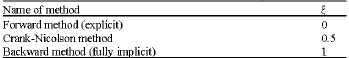 | |
Hydrodynamic model considers the left bank, the right bank and the main channel. Manning`s equation has been used to determine the friction slope. Friction slope has been assumed to be equal in the left bank, the right bank and the main channel in each section.
Equivalent Manning`s coefficient is calculated by Horton-Einstein equation.
(6) |
| pi | = | Wetted perimeter in each part |
| ni | = | Manning`s coefficient in each part |
| ne | = | Equivalent Manning`s coefficient for cross section |
4-diagonal matrix is solved by Gauss elimination method. This method converts this matrix to an upper diagonal matrix.
The stochastic part of model produces boundary conditions for the hydrodynamic part of model.
c) Advection-diffusion equation is applied for determination of the salinity concentration. Perfect form of the advection-diffusion equation is shown as follow:
(7) |
Equation 7 is a 3-D equation. 1-D model applied to the rivers because the length of the rivers is very larger than the width and the depth of the rivers. 1-D form of Eq. 7 is
(8) |
(9) |
Where:
(10) |
| C | = | Salinity concentration (mg L-1) |
| U | = | Current velocity in longitude direction of the river (m sec-1) |
| D | = | Salinity distribution coefficient in longitude direction of the river (m2 sec-1) |
| t | = | Time step (sec) |
| x | = | Distance between consecutive sections (m) |
For solving to Eq. 8, it makes use of Preissman method.
Salinity distribution coefficient for the tidal rivers: Based on the amount of the fresh water discharge and the range of tidal height in the tidal rivers, it is two states.
| • | If the range of tidal height in the mouth of tidal river is high and the discharge of fresh water is low, tidal rivers will have fully stratification state. |
In this state, stream of river has two distinguished layer. In the lower layer, the salinity concentration is equal to the salinity concentration of the sea. In the upper layer the salinity concentration is equal to the salinity concentration of fresh water. Between two layers is a distinguished boundary. Velocity on distinguished boundary is zero and two layers do not combine with another and turbulent effects are lower than gravity effects.
| • | If the range of tidal height in the mouth of tidal river is low and the discharge of fresh water is high, tidal rivers will have well mixed state. |
In this state, the difference between the salinity concentration in water surface and the salinity concentration in top of bed of river is lower than fifty percent of the average of salinity concentration in cross section. There is not a distinguished boundary in this state. Turbulent effects are higher than gravity effects.
If a 3-D model is applied to determination of the salinity concentration of the tidal rivers, it can make use of ordinary distribution coefficient while 1-D models need to increase of the salinity distribution coefficient in order to they can consider different states of the tidal rivers (especially fully stratification state).
Based on above concept, the salinity model part of model makes use of following procedure for determination of the salinity distribution coefficient.
| • | Calculation of the salinity distribution coefficient that is similar to the no tidal river in this stage. Following formula is applied for this stage: |
(11) |
| n | = | Manning`s coefficient |
| R | = | Hydraulic radius (m) |
| • | Using of the characteristics of tidal surges (domain and period of the tidal surges) |
| • | Using of suitable formulas for correction of the distribution coefficient. These formulas are shown as follow: |
(12) |
(13) |
(14) |
(15) |
| T | = | Period time of tidal surge (sec) |
| ω | = | Frequency of tidal surge (rad sec-1) |
| a | = | Domain of tidal surge (m) |
| g | = | Gravity acceleration (m sec-2) |
| Uf | = | The velocity of fresh water (m sec-1) |
| Dx | = | Modified distribution coefficient for the tidal rivers (m2 sec-1) |
| G | = | The tidal energy dissipation rate per unit mass (m2 sec-3) |
| J | = | The gain of potential energy rate per unit mass (m2 sec-3) |
Dx, G and J are functions of time and distance of the mouth of the tidal river.
Constant in Eq. 15 is determined by calibration of salinity part model and is a function of distance from the mouth of the tidal rivers.
The salinity part of model is run for two steps:
| • | In this step, model is run for the average tidal height in the mouth of the tidal river, this step results Uf. In this step the effects of fresh water are considered and tidal surges are ignored. |
| • | In this step, model is run for general conditions and the effects of fresh water and the effects of tidal surges are considered. In the other words tidal cycle is applied for downstream boundary conditions. |
The salinity concentration is equal to zero for initial conditions. Because the distribution coefficient depends on the salinity concentration, this model makes use of trial-error method. This procedure is repeated until reach to convergence. At the first, the salinity concentration is assumed that is equal to the salinity concentration in the former time step.
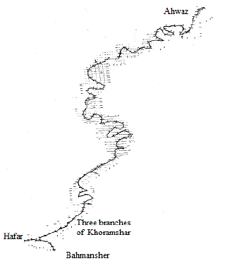 | |
| Fig. 1: | The Karun river |
This model is a general model for tidal rivers. In this research, model applied for the Karun River in Iran. Results show that this model is a suitable model for comprehensive hydraulic analysis in tidal rivers.
The Karun river: The Karun River is the most important tidal river in Iran. Selected reach in this river is between the hydrometric station of Ahvaz in upstream and three branches of Khoramshar in downstream. This reach has 145 cross sections (Fig. 1). Time of simulation is equal to 24 h and length of the reach is 188.760 km.
Manning`s coefficient is determined by calibration of hydrodynamic part of model for different parts of the reach. The range of Manning`s coefficient is 0.015 to 0.057.
Joint probability of tidal surges and discharges of fresh water in The Karun river: Governing stochastic distribution on annual minimum discharges is person III distribution in the hydrometric station of Ahvaz.
For different return periods, minimum discharges of fresh water are shown in Table 2.
Governing stochastic distribution on annual maximum tidal elevation is Gumbel distribution in three branches of Khoramshar.
For different return periods, tidal elevations are shown in Table 3.
The lowest discharges of fresh water and the highest tidal surges of the Karun River occur in June and July.
| Table 2: | Minimum discharges of fresh water for different return periods in the hydrometric station of Ahvaz |
| Table 3: | Tidal elevations for different return periods in three branches of Khoramshar |
Because the discharge of the Karun River is almost constant in June and July, the highest tidal surge occur contemporary to the lowest discharge. Therefore combination coefficient of the tidal surge and the minimum discharge of fresh water is equal to one.
RESULTS
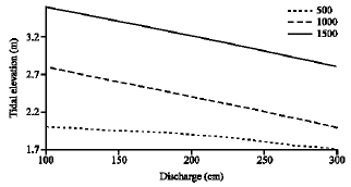
Results of hydrodynamic part of model for The Karun river: For boundary conditions in joint probability analysis, this model make use of a constant discharge of fresh water in upstream boundary and an indicator tidal height hydrograph in downstream boundary. This hydrograph is shown in Fig. 2 for Karun River.
For producing a tidal height hydrograph, maximum tidal height of considerable tidal surge is divided to maximum tidal height of indicator tidal surge. Then, this relation multiplies to tidal heights of indicator tidal surges.
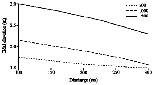
Water surface elevations for different combinations of discharges of fresh water and tidal surges are shown in Fig. 3.
Results of salinity part of model for The Karun river: The salinity concentration is determined for different combinations of discharges of fresh water and tidal surges.
The observation stations are situated at Salmanieh and Darkhovein at 160 and 140 km from the Ahvaz hydrometric station, respectively.
For boundary conditions and salinity concentration in Darkhovein and Salmanieh stations, model makes use of the following regression relation:
(16) |
| Q | = | Discharge of fresh water (CMS) |
| H | = | Height of water surface elevation in considerable station (m) |
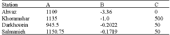
The values of a, b, c are shown in Table 4 for different stations.
This model is applied for different combinations of discharges of fresh water and tidal surges.
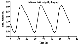 | |
| Fig. 2: | Indicator tidal height hydrograph in the Karun river |
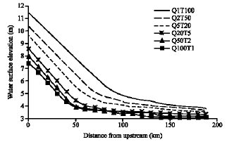 | |
| Fig. 3: | Maximum water surface elevation for different combinations of discharges of fresh water and tidal surges |
| Table 4: | Values of a, b, c in different stations |
 | |
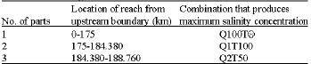
| Table 5: | Governing combination for different section of the Karun River |
 | |
Maximum salinity concentration is shown in Fig. 4 for different combinations.
Combinations that produce maximum salinity concentration in different sections are shown in Table 5.
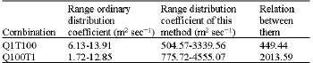
Comparison between the ordinary distribution coefficient and the distribution coefficient of this method is shown in Table 6.
The results of salinity part of model are compared to regression data in Darkhovein and Salmanieh stations in the Karun River. Mean of regression relations for different combinations of discharges of fresh water and tidal surges are 0.839 for Darkhovein Station and 0.946 for Salmanieh Station.
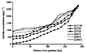 | |
| Fig. 4: | Maximum salinity concentration for different combinations of discharges of fresh water and tidal surges |
 | |
| Fig. 5: | Salinity curve for Darkhovein station |
 | |
| Fig. 6: | Salinity curve for Salmanieh station |
| Table 6: | Comparison between ordinary distribution coefficient and distribution coefficient of this method |
 | |
Salinity curves for Darkhovein and Salmanieh are shown in Fig. 5 and 6.
DISCUSSION
By decrease of the fresh water discharge, relation between ordinary distribution coefficient and the distribution coefficient of this method and the distribution coefficient of this method increases because the fully stratification state occurs. By increase of the fresh water discharge, the ordinary distribution coefficient increases because the ordinary distribution coefficient is a function of current velocity while the distribution coefficient of this method decrease.
By observation of salinity curve, tidal surges are governing factor in salinity concentration of the downstream of the Karun River. If tidal height is low in mouth of the tidal river, discharge of fresh water will effect salinity concentration.
CONCLUSION
The developed method in this research is a suitable method for determining the salinity concentration of the tidal rivers because different factors (domain and period of tidal surges, the salinity concentration, velocity of fresh water, velocity of tidal surges, area of cross sections and Manning`s coefficient) are considered for determine of the distribution coefficient. For determination of salinity concentration, it has to be considered different combinations of discharges of fresh water and tidal surges. Joint probability method is a suitable method that considers different combinations and shows combination that produces maximum salinity concentration in different sections of the tidal rivers and different time steps.
REFERENCES
- Acreman, M.C., 1994. Assessing the joint probability of fluvial and tidal floods in the river roding. J. Water Environ., 8: 490-496.
Direct Link - Causon, D.M., C.G. Mingham and D.M. Ingram, 1999. Advances in calculation methods for supercritical flow in spillway channels. J. Hydrol. Eng. ASCE., 125: 1039-1050.
Direct Link - Cheng, R.T., V. Casulli and J.W. Gartner, 1993. Tidal residual, intertidal mudflat (TRIM) model and its application to San Francisco Bay. Calif. Estuarine Coastal Shelf Sci., 36: 235-280.
Direct Link - Dawson, C.W. and R. Wilby, 1998. An artificial neural network approach to rainfall-runoff modelling. J. Hydrol. Sci., 43: 47-66.
CrossRefDirect Link - Gross, E.S., J.R. Koseff and S.G. Monismith, 1999. Evaluation of advective schemes for estuarine salinity simulations. J. Hydrol. Eng. ASCE., 125: 32-46.
CrossRefDirect Link - Huang, W. and M. Spaulding, 2000. Correlation of freshwater discharge and sub tidal salinity in Apalachicola River. J. Waterway Port Coast Ocean Eng. ASCE., 126: 264-266.
Direct Link - Jaffe, D.A. and B.F. Sanders, 2001. Engineered levee breaches for flood mitigation. J. Hydrol. Eng. ASCE., 127: 471-479.
Direct Link - Mantz, P.A. and H.L. Wakeling, 1979. Forecasting flood levels for joint events of rainfall and tidal surge flooding using extreme value statistics. Proc. Sin Civ. Eng., 67: 31-50.
CrossRefDirect Link - Mingham, C.G. and D.M. Causon, 1998. High-resolution finite volume method for shallow-water flows. J. Hydrol. Eng. ASCE., 124: 605-614.
CrossRefDirect Link - Naidu, V.S. and R.V. Sarma, 2001. Numerical modeling of tide-induced currents in Thane creek, west coast of India. J. Waterway Port Coast. Ocean Eng. ASCE., 127: 241-244.
Direct Link - Park, K., J.H. Oh, H.S. Kim and H.H. Im, 2002. Case study: Mass transport mechanism in Kyunggi bay around Han River mouth, Korean. J. Hydrol. Eng. ASCE., 128: 257-267.
Direct Link - Piasecki, M. and N.D. Katopodes, 1999. Identification of stream dispersion coefficients by ad joint sensitivity method. J. Hydrol. Eng. ASCE., 125: 714-724.
CrossRef - Piasecki, M. and B.F. Sanders, 2002. Optimization of multiple freshwater diversions in well-mixed estuaries. J. Water Resour. Plann. Manage., 128: 74-84.
Direct Link - Punt, A.G., G.E. Millward and J.R.W. Harris, 2003. Modelling solute transport in the Tweed Estuary, UK using ECoS. J. Sci. Total Environ., 314-316: 715-725.
Direct Link - Samuels, P.G. and N. Burt, 2002. A new joint probability appraisal of flood risk. Sin Civ. Eng., 154: 109-115.
CrossRefDirect Link - Sanders, B.F. and N.D. Katopodes, 2000. Ad joint sensitivity analysis for shallow-water wave control. J. Eng. Mech., 126: 909-919.
CrossRefDirect Link - Sanders, B.F., C.L. Green, A.K. Chu and S.B. Grant, 2001. Case study: Modeling tidal transport of urban runoff in channels using the finite- volume method. J. Hydrol. Eng. ASCE., 127: 795-804.
Direct Link - Sanders, B.F. and M. Piasecki, 2002. Mitigation of salinity intrusion in well-mixed estuaries by optimization of freshwater diversion rates. J. Hydrol. Eng. ASCE., 128: 64-77.
Direct Link - Sobay, R.J., 2001. Evaluation of numerical models of flood and tide propagation in channels. J. Hydrol. Eng. ASCE., 127: 805-824.
Direct Link