
Yanshan Li
ATR National Key Lab. of Defense Technology, Shenzhen University, Shenzhen, 518060, China
Information Technology Journal
Year: 2012 | Volume: 11 | Issue: 7 | Page No.: 904-909


ABSTRACT
In order to select best bands from the hyperspectral image with high computation efficiency, this paper proposed a new bands selection algorithm of hyperspectral image using the hyperspectral derivative on Clifford manifold. It firstly analyze the hyperspectral image in the Clifford algebra which had high efficiency on computation and analysis. Firstly, it discusses the properties of the Clifford algebra and Clifford manifold. Secondly, it gives the definitions of the hyperspectral derivative and the curve change rate on high dimensional space in Clifford algebra for finding the key points. Based on the theories mentioned above, a new bands selection algorithm is given with detail steps. At last, the results of the experiments are shown. Compared with the existing algorithms, the proposed algorithm is highly efficient in respect of computation and time. The study provided a new method for bands selection algorithm of hyperspectral image with the theories of Clifford algorithm.
PDF Abstract XML References Citation
Received: November 05, 2011;
Accepted: March 28, 2012;
Published: May 29, 2012
How to cite this article
Yanshan Li, 2012. A New Bands Selection Algorithm for Hyperspectral Image using Hyperspectral
Derivative on Clifford Manifold. Information Technology Journal, 11: 904-909.
DOI: 10.3923/itj.2012.904.909
URL: https://scialert.net/abstract/?doi=itj.2012.904.909
DOI: 10.3923/itj.2012.904.909
URL: https://scialert.net/abstract/?doi=itj.2012.904.909
INTRODUCTION
With the development of the hyperspectral image processing technology, this technology has been applied to more and more fields, such as remote sensing (Landgrebe, 2000; Mazzoni et al., 2007), medicine (Rajpoot and Rajpoot, 2004), military, etc. The main reason is that the hyperspectral image can provide high spectral information which is useful for analyzing the composition of material. However, it contains huge redundant data. The redundant data not only increases the difficulty of data processing but also reduces the efficiency of data processing. Because the traditional image processing methods are developed on the 2D or 3D images, the traditional image processing method is not feasible for the high dimensional image. It is necessary to reduce the band size of the hyperspectral image. In recent years, the technology of hyperspectral image processing has become a new research hotspot of the image processing (Mianji et al., 2009; Mianji et al., 2008; Windham et al., 2005; Misman et al., 2010). This study introduces the Clifford algebra theory for hyperspectral image processing to provide a new way.
Bands selection is a very important way to reduce the dimension of hyperspectral image besides the feature extraction. It figures out the bands subset of hyperspectral data. The selected bands yield the best performance based on some criteria which are usually linked to some measure of end-performance. Compared to the feature extraction, bands selection has advantage of saving the original information of the bands. There are many algorithms presented for feature selection. The Jeffreys-Matusita distance (JM-distance) (Swain and King, 1973; Bruzzonne et al., 1995) is proposed based on divergence and it derives two criteria, the average separability criterion and the saturating transform of divergence for bands election. Keshava (2001) quantifies the distance between the spectra of two materials at corresponding spectral bands and then analyzes the separability of these two spectra using the Spectral Angle Mapper (SAM) metric. The spectral bands are selected in order to maximize the SAM metric, that is, the angle between the two spectra. Stein et al. (1999) apply Spectral Matched Filter (SMF) which is the likelihood ratio detection statistics for a known additive signal in a Gaussian background. They then evaluate the SNR losses and select spectral bands in order to optimize an objective function which is defined in terms of probability of detection. Kira and Rendell (1992) assign weights to features individually to indicate their relevance to a given task and select features with greater weights. Briefly, these algorithms including many other bands selection algorithms have good performance in specified tasks. The feature selection method based on Hybrid Genetic Algorithm (HGA) can select feature subsets which not only contain fewer features but also provide better detection performance for steg-analysis (Xia et al., 2009). However, there are still some challenges in applying these techniques effectively, such as computational cost, timely cost and presence of local minima problems, etc. This study try to develop a new bands selection algorithm with less computational cost and timely cost based on Clifford algebra.
CLIFFORD ALGEBRA
Basic of Clifford algebra: Clifford algebra (Li et al., 2001; Sommer, 1998; Penrose and Rindler, 1984) provides an efficient framework to conduct the computations without coordinates. It can reduce the computation complexity and improve the efficiency of the computation. This algebraic approach contains all geometric operators and permits specification of constructions in a coordinate-free manner. It has widely been used in physics (Byrnes, 2006), computer vision (Schlemmer, 2004; Brackx and Schepper, 2005; Yanshan, 2008) and so on, due to two main advantages detailed as follows (Batard et al., 2009):
| • | Clifford algebra is generally known that Clifford algebra provides a very efficient framework to conduct computations without coordinates. It can be used in the inner, wedge and geometric products as well as the related geometric interpretations of these operations. More precisely, the acquisition space of the image, i.e. the space where the image gets its values, is embedded into Clifford algebra. The local variations of the pixel values can be easily measured using geometric information and transformations |
| • | Clifford algebra provides very convenient ways for computing in high dimensional space. Clifford algebra contains elements of different degrees (scalar, vectors, bivector, pseudoscalar, etc.). This allows combining information of different natures in a single multivector which process data as a global and concise way |
Let ![]() be n-dimensional Euclidean space, with the positive definite inner product 〈.,.〉.
be n-dimensional Euclidean space, with the positive definite inner product 〈.,.〉. ![]() has an orthogonal basis e1, e2,…, en, such that〈ei, ej〉= δij.
has an orthogonal basis e1, e2,…, en, such that〈ei, ej〉= δij.
The Clifford algebra α(![]() , n) is the free algebra generated by
, n) is the free algebra generated by ![]() modulo as the relation:
modulo as the relation:
| (1) |
It can be considered as being the exterior algebra ∧![]() , where the extra information defining the inner product is included. From this point of view one has:
, where the extra information defining the inner product is included. From this point of view one has:
| (2) |
for arbitrary vectors. Clearly, for n>1, α(![]() , n) is not commutative.
, n) is not commutative.
For practical reasons, it can simple α(![]() , n) to α(n) which then contains elements of the form a+ib.
, n) to α(n) which then contains elements of the form a+ib.
where, a and b are from α(![]() , n). Multiplication then assumes that i commute with all elements of the Clifford algebra. Based on α(n) we can define an anti-automorphism by:
, n). Multiplication then assumes that i commute with all elements of the Clifford algebra. Based on α(n) we can define an anti-automorphism by:
| (3) |
for arbitrary x in ![]() and a and b in α(n). There is a natural identification of
and a and b in α(n). There is a natural identification of ![]() as a subspace of the finite-dimensional algebra α(n) and the scale part in a Clifford number is clearly presented which will be denoted as [a]0.
as a subspace of the finite-dimensional algebra α(n) and the scale part in a Clifford number is clearly presented which will be denoted as [a]0.
Clifford manifold: A vector manifold (Hestenes and Sobczyk, 1984) M is a set of vectors called points of M with certain properties to be described presently. A vector a(x) is said to be tangent to a point x in M if there is a curve {z(τ); 0<τ<ε} in M extended from the point x(0) = x such that:
| (4) |
If the chord of a curve are not null vectors, the curve can be parameterized by the magnitudes of its chords, σ = σ(τ)≡|x(τ)-x|, so:
The set A(x) of all vectors tangent to M at x is called the tangent space at x. At each interior point x of M, the tangent space A(x) is an m-dimensional vector space and M denotes an m-dimensional manifold.
The tangent space A(x) at an interior point generates a unique Clifford algebra which we call the tangent algebra of M at x and denote by G (x)≡G(A(x)). We assume that A(x) is nonsingular in the algebraic sense that it possesses a unit pseudoscalar I = I(x) which we call the (unit) pseudoscalar of M at x.
HYPERSPECTRAL DERIVATIVE IN α(![]() , n)
, n)
Representation for hyperspectral data set: The spectrum recorded is a combination of the actual spectrum of the real surface, modulated by the effects of the solar curve and the complexity of the ground. The spectrums of the points belonged to same class are usually different, since the effects on different points are different. Figure 1 shows the spectrums of the points selected from the water area.
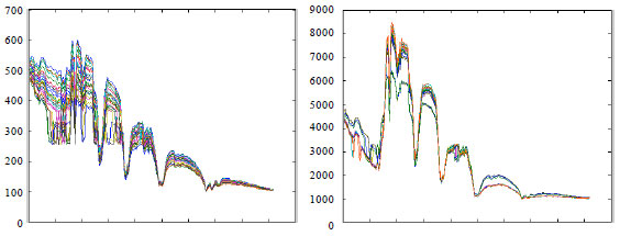 | |
| Fig. 1: | The spectral curves of some materials. Every point of the hyperspectral image form a individual curve, one material always forms many curves |
It is apparently that the curves belonged to a same material are different and It is also shown that just only using one spectrum of one point or the average spectrums value of one class can hardly represent the whole spectral property of one class. In our work, we represent the data belonged to one class with a curve in high dimensional space, so the spectral properties of all samples can entirely be used in the feature selection.
Let us consider a hyperspectral image with C class labels and n spectral bands. We represent the data from one class with a curve in high dimensional space, so it produces C curves in the space whose dimension is the maximum count of the samples in classes.
Given a set of samples ![]() , xi is the pixel of the hyperspectral image. We define a map function
, xi is the pixel of the hyperspectral image. We define a map function ![]() , where m is the maximum count of the samples in classes. We assume that there are C curves on the manifold M, denoted by fi, where 1≤i≤C. The curve fi include the samples labeled by class i, denoted by S = {s1, x2,…, sd}, where si = Bi(xc1)e1+Bi(xc2)e2+…+Bi(xcm)em and Bi(xcm) represents the ith band of the pixel xcm. The tangent space is denoted by A(x).
, where m is the maximum count of the samples in classes. We assume that there are C curves on the manifold M, denoted by fi, where 1≤i≤C. The curve fi include the samples labeled by class i, denoted by S = {s1, x2,…, sd}, where si = Bi(xc1)e1+Bi(xc2)e2+…+Bi(xcm)em and Bi(xcm) represents the ith band of the pixel xcm. The tangent space is denoted by A(x).
Hyperspectral derivative in α(![]() , n): The normal first order derivative can be estimated by:
, n): The normal first order derivative can be estimated by:
| (5) |
where, the s is the spectral function, λi is the wavelength of the ith band, s(λi) is the reflectance value at wavelength λi, Δλ = λj-λi and λj>λi.
From the hyperspectral curve in α(![]() , n), we give the definition of the first order derivative as below:
, n), we give the definition of the first order derivative as below:
| (6) |
where, S is the high dimensional curve of some samples with same class label, D(.) is the distance metric function between the S(λi) and S(λj) and Δλ = λj-λi.
There are many distance metric existed in high dimensional space. In this study, we use the distance metric function based on the Clifford algebra as follows:
| (7) |
Using Eq. 6, one can compute derivatives of the hyperspectral image simply and identify the derivative features of one target classes. These features can then be included in the bands or feature selection operation to improve the efficiency. It is important to remember that no new information is created by using derivatives. The purpose is to identify the helpful spectral features that may be too subtle to be captured by other methods, so that the data dimension of the image can be kept, also was possible and still achieve accurate classification results.
BANDS SELECTION ALGORITHM USING HYPERSPECTRAL DERIVATIVE
Key points of hyperspectral curve: Suppose pixels belonging to one target class form a curve on the Clifford manifold, there must be many points which can identify the curve from other curves belonging other classes. These points are called key points in this study. the key points are noted by Xkey = {xkey1, xkey2,…, xkeyk}⊂X. In order to determine whether a band point is a key point, a criterion is defined by:
 | (8) |
where, CR(xi, xj) = |S| and ∀xi, xj, xcεX) belong to one target class.
Equation 8 can only give the geometric features of one class but it can not measure the separability of two classes. In order to select out the appropriate bands, the separability measure is necessary. In this study the separability measure of a point xc among classes can be computed by:
| (9) |
Algorithm: Suppose that the training data set contains d classes and n bands, k optimal bands is required to be selected. Xkey = {xkey1, xkey2,…, xkeyk}⊂X is the set of the key points and Xs = {xs1, xs2,…, xsm}⊂X is the selected band points. So, The detailed steps of bands selection framework is as below.
 |
EXPERIMENTAL RESULTS AND ANALYSIS
Dataset description: The hyperspectral dataset used in our experiments is a section of a scene taken over northwest Indiana’s Indian Pines by the AVIRIS sensor in 1992. From the 220 spectral channels acquired by the AVIRIS sensor, 20 channels were discarded because affected by atmospheric problems. From the 16 different land-cover classes available in the original ground truth, seven were discarded; since only few training samples were available for them (this makes the experimental analysis more significant from the statistical viewpoint). The remaining nine land-cover classes were used to generate a set of 4757 training samples (used for learning the classifiers) and a set of 4588 test samples (exploited for assessing their accuracies). The experiments were run on a computer with Intel core 2 Dou CPU E7400.
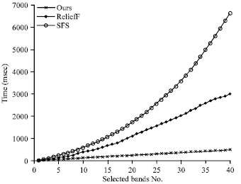
Experimental results and analysis: Several experiments with many different bands selection algorithms are completed on the same hyperspectral image. Figure 2 shows the experimental result of different bands selection algorithms including the proposed framework, Sequential Forward Selection (SFS) and ReliefF. It shows that all the average recognition correct rates using the Bayesian classification on the selected bands. The recognition correct rate are raised when the number of the selected bands is rising. The rate of our method is higher than the SFS and ReliefF, especially when the number of the selected bands is small. Figure 3 shows the time cost of our algorithm, SFS and ReliefF.
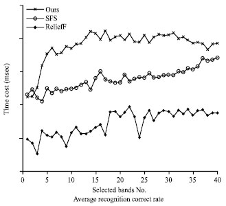 | |
| Fig. 2: | The time cost of ours, SFS and ReliefF |
 | |
| Fig. 3: | Average recognition correct rates algorithm, using the Bayesian classification on the selected bands which selected by our algorithm, SFS, and ReliefF |
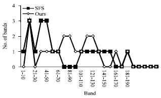 | |
| Fig. 4: | Distribution of the selected bands |
It is apparent that the time cost of our algorithm is smaller than the other algorithms and with the number of selected bands rising, the advantage of our algorithm in the time cost is more and more greater. When the number of selected band is 40, the time cost of our algorithm is about 17% of the ReliefF and about 8% of the SFS.
Figure 4 shows the distribution of the selected bands by our method and SFS. It shows that the selected bands are distributed evenly on the whole spectrum.
CONCLUSIONS
This study proposed a new bands selection algorithm for hyperspectral image using the hyperspectral derivative on Clifford manifold. Firstly, the properties of the hyperspectral image in the Clifford algebra are analyzed and then a new bands selection algorithm for hyperspectral image is represented. Compared with the existing algorithm, the proposed algorithm reduces the computational time considerably. However, there are still many further studies worth to do, including the analysis technologies with Clifford algebra theories, Clifford manifold theories, bands selection algorithm in high dimension space and so on.
REFERENCES
- Mazzoni, D., M.J. Garay, R. Davies and D. Nelson, 2007. An operational MISR pixel classifier using support vector machines. Remote Sens. Environ., 107: 149-158.
CrossRef - Mianji, F.A., Y. Zhang and A. Babakhani, 2009. Optimum method selection for resolution enhancement of hyperspectral imagery. Inform. Technol. J., 8: 263-274.
CrossRefDirect Link - Keshava, N., 2001. Best bands selection for detection in hyperspectral processing. Acoustics Speech Signal Process., 5: 3149-3152.
CrossRefDirect Link - Xia, Z., X. Sun, J. Qin and C. Niu, 2009. Feature selection for image steganalysis using hybrid genetic algorithm. Inform. Technol. J., 8: 811-820.
CrossRefDirect Link - Mianji, F.A., Y. Zhang, H.K. Sulehria, A. Babakhani and M.R. Kardan, 2008. Super-resolution challenges in hyperspectral imagery. Inform. Technol. J., 7: 1030-1036.
CrossRefDirect Link - Windham, W.R., D.P. Smith, M.E. Berrang, K.C. Lawrence and P.W. Feldner, 2005. Effectiveness of hyperspectral imaging system for detecting cecal contaminated broiler carcasses. Int. J. Poult. Sci., 4: 657-662.
CrossRefDirect Link - Misman, M.A., H.Z.M. Shafri and R.M.K.R. Ahmad, 2010. Effects of hyperspectral data transformations on urban inter-class separations using a support vector machine. J. Applied Sci., 10: 2241-2250.
CrossRef - Batard, T., C. Saint-Jean and M. Berthier, 2009. A metric approach to nD images edge detection with clifford algebras. J. Math. Imag. Vision, 33: 296-312.
CrossRefDirect Link - Bruzzonne, L., F. Roli and S.B. Serpico, 1995. An extension of the Jeffreys-Matusita distance to multiclass cases for feature selection. IEEE Trans. Geosci. Remote Sens., 33: 1318-1321.
CrossRef