
Mitat Uysal
Department of Computer Engineering, Dogus University, Acibadem, Kadikoy, Istanbul, Turkey
Information Technology Journal
Year: 2007 | Volume: 6 | Issue: 3 | Page No.: 475-477


ABSTRACT
In this resarch, Radial Basis Function Networks (RBFN) and ARIMA models(Autoregressive Integrated Moving Average) are compared to their ability to predict time series values.RBFN gives good results in many cases but for some extreme values of time series, better approximations can be obtained using ARIMA models.
PDF Abstract XML References Citation
How to cite this article
Mitat Uysal, 2007. Comparison of ARIMA and RBFN Models to Predict the Bank Transactions. Information Technology Journal, 6: 475-477.
DOI: 10.3923/itj.2007.475.477
URL: https://scialert.net/abstract/?doi=itj.2007.475.477
DOI: 10.3923/itj.2007.475.477
URL: https://scialert.net/abstract/?doi=itj.2007.475.477
DESCRIPTION OF THE PROBLEM
In real world applications, many processes can be represented using time series models as below:
For making a prediction using time series, a large variety of approaches are available. Prediction of scalar time-series {x(n)} refers to the task of finding an estimate ![]() of the next future sample x(n+1) based on the knowledge of the history of time-series, i,e., the samples x(n), x(n-1), … (Rank, 2003).
of the next future sample x(n+1) based on the knowledge of the history of time-series, i,e., the samples x(n), x(n-1), … (Rank, 2003).
Linear prediction, where the estimate is based on a linear combination of N past samples can be represented as below:
with the prediction coefficients αi, i = 0,1, … N-1.
Introducing a general nonlinear function f(·); ![]() applied to the vector x(n) = [x(n), x(n - M), …, x(n-(N-1))M]T of past samples, we arrive at the nonlinear prediction approach
applied to the vector x(n) = [x(n), x(n - M), …, x(n-(N-1))M]T of past samples, we arrive at the nonlinear prediction approach ![]() (Rank, 2003).
(Rank, 2003).
ARIMA MODEL
Traditionally, time series forecasting problem is tackled using linear techniques such as Auto Regressive Moving Average (ARMA) and Auto Regressive Integrated Moving Average (ARIMA) models popularized by Box and Jenkins (1976).
The general form of ARMA(p,q) model can be written as below:
where {εt} is white noise. This process is stationary for appropriate φ, θ (Box and Tenkins, 1976).
The general form of the ARIMA model is given by:
I = 1, 2, …YYp and j = 0, 1,…YY. Q |
where Yt is a stationary stochastic process with non-zero mean, a0 is the constant coefficient, ei the white noise disturbance term, ai represents autoregressive coefficients and bj denotes the moving average coefficients.
RADIAL BASIS FUNCTION NETWORK
The RBF network consists of 3 layers: an input layer, a hidden layer and an output layer. A typical RBF network is shown in Fig. 1.
Mathematically, the network output for linear output nodes can be expressed as below:
Where x is the input vector with elements xi (where i is the dimension of the input vector); ![]() is the vector to determine the center of the basis function; φj with elements ; Wkj‘s are the weights and Wko is the bias (Duy and Cong, 2003). The basis function φj(-) provides the non-linearity.
is the vector to determine the center of the basis function; φj with elements ; Wkj‘s are the weights and Wko is the bias (Duy and Cong, 2003). The basis function φj(-) provides the non-linearity.
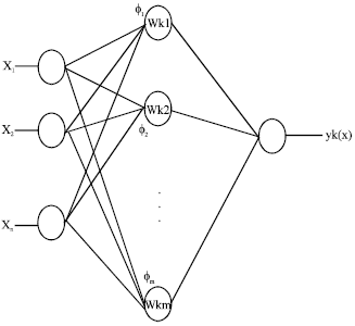 | |
| Fig. 1: | Typical RBF network |
BASIS FUNCTIONS
The most used basis functions are Gaussian and multiquadratic functions. They are given below:
| • | Gaussian φ(x) = exp(-x2/2δ2) for δ > 0 and x ε |
| • | Multiquadratic φ(x) = (x2+δ2)p for δ > 0 and xε |
CALCULATING THE OPTIMAL VALUES OF WEIGHTS
A very important property of the RBF Network is that it is a linearly weighted network in the sense that the output is a linear combination of m radial basis functions, written as below:
The main problem is to find the unknown weights
For this purpose, the general least squares principal can be used to minimize the sum squared error:
With respect to the weights of f, resulting in a set of m simultaneous linear algebraic equations in the m unknown weights (ATA) w = Aty
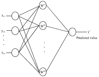 | |
| Fig. 2: | Finding predicted value yt |
Where
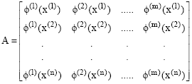 |
In the special case where n = m, the resultant system is just Aw = y (Duy and Cong, 2003).
The output y(x) represents the next value of y in time t taking input values x1, x2, …, xn that represent the previous function values set with values yt-1, yt-2, …, yt-n. So, xn corresponds to yt-1, xn-1 corresponds to yt-2 etc. as in Fig. 2.
SIMULATION RESULTS
For this work, the time series data of American Express Bank is used. Monthly log data consists of 324 data items. The first 162 data items are used for training and the remaining 162 data items are used for forecasting.
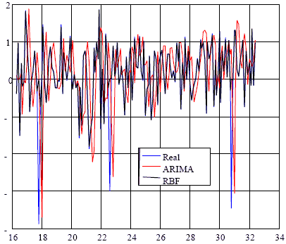
Figure 3 shows the results of simulation run with σ = 1.5 and 18 neurons in the hidden layer of the Radial Basis Function Network with the results of ARIMA model for the same data.
As in Fig. 3 and 4, RBFN approach provides better results than ARIMA model in a big part of data interval except the peak points.
In this points, ARIMA model gives better results than RBFN approach.
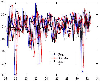 | |
| Fig. 3: | Simulation Results for ARIMA and RBFN models |
 | |
| Fig. 4: | Simulation results for ARIMA and RBFN models with a different format |
CONCLUSIONS
Radial Basis Functions Networks provide a good way to predict the future values in a time series. In the peak points of the original data, ARIMA model gives better results than RBFN approach.
In order to obtain the best results of the whole interval of the data, a hybrid model that consists of ARIMA and RBFN approach can be used to predict the future values of the time series.
REFERENCES
- Duy, N.M. and T.T. Cong, 2003. Approximation of function and its derivations using radial basis function networks. Applied Math. Modell., 27: 197-220.
Direct Link - Rank, E., 2003. Application of bayesian trained RBF networks to nonlinear time-series modeling. Signal Process., 83: 1393-1410.
Direct Link