
S.K. Balasundram
Not Available
P.C. Robert
Not Available
D.J. Mulla
Not Available
D.L. Allan
Not Available
Asian Journal of Plant Sciences
Year: 2006 | Volume: 5 | Issue: 2 | Page No.: 397-408


ABSTRACT
This study reports on the spatial variability of soil fertility variables influencing oil palm yield in small-scale plots situated at varying topographic positions. For each topographic position, Yield-influencing Variables (YIVs) were determined and subjected to spatial data analyses involving variography and interpolation (inverse distance weighting). Results showed that the spatial structure of YIVs differed across topographic positions. The optimum sampling strategy was found to depend on the type of variable being investigated and its topographic position. A management zone concept with topography as the delineation factor seemed appropriate for fertility management. Only potassium (K) showed a clear demarcation of zones with high, moderate or low values and hence the need for variable rate management.
PDF Abstract XML References Citation
How to cite this article
S.K. Balasundram, P.C. Robert, D.J. Mulla and D.L. Allan, 2006. Spatial Variability of Soil Fertility Variables Influencing Yield in Oil Palm (Elaeis guineensis Jacq.). Asian Journal of Plant Sciences, 5: 397-408.
DOI: 10.3923/ajps.2006.397.408
URL: https://scialert.net/abstract/?doi=ajps.2006.397.408
DOI: 10.3923/ajps.2006.397.408
URL: https://scialert.net/abstract/?doi=ajps.2006.397.408
INTRODUCTION
Variation in soil properties (Brubaker et al., 1993; Cassel et al., 1996), crop yields (Verity and Anderson, 1990; Mahli et al., 1993) and fertilizer response (Nolan et al., 1995) over the landscape is well established. Results from these studies validate the recommended strategy of apportioning more resources at lower slope positions (Kachanoski et al., 1985) where yield potential is greatest.
In order to understand soil spatial variability, it is common to collect extensive soil samples. Often this exercise poses a cost constraint. Depending on field variability, the number of samples per ha ranges from 25 to 50 for hydraulic conductivity, 7 to 14 for infiltration rate and 24 to 55 for determining solute concentration (Hajrasuliha et al., 1980; Gajem et al., 1981; Vieira et al., 1981). Additionally, the large degree of spatial variation in the field necessitates collection of soil samples from closer spacing in order to obtain an accurate estimate of a soil property. Sampling intervals as small as 1 m for hydraulic conductivity, 0.05 to 2 m for infiltration rate and 0.2 to 80 m for electrical conductivity have been suggested (Russo and Bresler, 1981; Sisson and Wierenga, 1981). Spatial variability in soil properties inevitably affects the efficiency of input (i.e., fertilizers, pesticides) use within a field. Studies have shown that such variability often justifies variable fertilizer recommendation, which is based on the nutrient requirements of a specific site, rather than a uniform fertilizer recommendation for the entire field (Carr et al., 1991).
Quantifying the spatial variability of soil properties and/or crop yield is an important pre-requisite when considering site-specific applications, more so for cropping systems that are established on rolling topography.
The Republic of Indonesia ranks number two in global palm oil production and has the fastest growing palm oil sector in the world (Mielke, 1998). Approximately 70% of oil palm cultivation in Indonesia is concentrated in the island of Sumatra (ARAB, 2000). The need for site-specific practices in oil palm plantations is mainly driven by stagnant productivity and increasing input costs over the past 20 years. Fertilization is often reported as the biggest cost component (35-50%) in the operating budget. The concept of site-specific nutrient management appears as an attractive solution to offset this existing dilemma.
Currently, there is limited information about the spatial variability in oil palm yield or its soil fertility and how soil spatial variation impacts sampling strategy. In the context of plantation-based oil palm, such information will allow the demarcation of a field into clusters of palms where palms are spatially related within each cluster but independent between clusters. Thus, each cluster of palms is unique and can be managed separately for optimum returns. Technically, this approach is known as management zoning.
Hence, this study was aimed at quantifying the spatial variability of soil fertility variables influencing oil palm yield in small-scale plots situated at varying topographic positions.
MATERIALS AND METHODS
Study location and site attributes: This study was carried out in Sungai Lilin, South Sumatra, Indonesia. The study site, Sri Gunung Estate, is geographically located at 02° 31’ South and 104° East and is characterized by rolling topography with 4-12% slope (Fig. 1). The area planted to oil palm in Sri Gunung is 887 ha. The palm trees are planted in an equilateral triangular pattern resulting in all palms being equidistant from one another. Planting and inter-row distances are typically 9.1 and 7.9 m, respectively. This translates into a planting density of 136 palms per ha. The annual rainfall at Sri Gunung ranges from 3000 to 3200 mm annually.
Plot layout: The study site was partitioned into three observational plots that were established based on topography; one plot each at the toeslope (0.88 ha), sideslope (3.44 ha) and summit (1.15 ha) position. All observation plots comprised single-variety palms that were field-planted in January of 1998.
Each plot featured two adjacent blocks that were divided by a collection road. The number of palms chosen to represent an observation strip was based on the plantation’s standard harvesting procedure comprising 13 palms per strip per block. Two strips of palms per block were designated as an observation unit bearing a dimension of 8x119 m. A total of 3 observation units (6 strips) were established on each block for the toeslope and summit plots. For the sideslope plot, 3 observation units on both adjacent blocks constituted a replicate. The sideslope plot consisted of 3 replicates.
Sampling protocol: Three composite samples were obtained from each observation unit using a systematic scheme. Each leaf sample was made up of four sub-samples obtained from the central leaflets of frond number 17. Each soil sample was made up of six sub-samples taken randomly at 0-20 cm and 20-40 cm depths outside the fertilizing circle, the area girdled beneath the palm canopy. Within each plot, sample points were spaced 36.4 m apart between palms (x direction) and 8.7 m apart between strips (y direction). Leaf and soil samples were obtained 2 months after standard routine fertilization at a 6-month interval over 2 years. A total of 30 samples were obtained at the toeslope and summit positions while the sideslope position afforded 54 samples.
Yield and fertility measurements: Oil palm yields were recorded in situ for each observation unit based on the standard 10-day harvest interval and then averaged to give a monthly count expressed as kg fresh fruit bunch (FFB) per palm. Leaf analysis was performed to quantify N, P, K, Mg and Ca while soil analysis was carried out to determine pH, organic carbon (C), extractable P, exchangeable K, Mg and Ca, Effective Cation Exchange Capacity (ECEC) and texture.
Bivariate relationships were explored using Pearson correlation and backward stepwise multiple linear regression. The difference in leaf/soil variables and yield as a function of topographic position was determined using analysis of variance followed by mean separation using the Least Significant Difference (LSD) criterion. Empirical production functions based on measured leaf/soil variables as well as leaf/topsoil nutrient ratios were defined for each topographic position at both study sites.
Geo-spatial data analysis: Geo-spatial description of the data was performed in two stages: 1) spatial continuity analysis using variography and 2) interpolation using inverse-distance weighting (IDW). The toeslope and summit positions were represented by 30 observations, while the sideslope had 54 observations. To perform kriging, the minimum number of observation pairs required is 30, which effectively translates to more than 30 observation points (Journel and Huijbregts, 1978). According to Whelan et al. (1996), IDW is more effective than kriging when interpolating based on a small number of observations collected at moderate intensity. In either event, the data should still display spatial dependency. Webster and Oliver (1992) showed how sensitive the variogram is to sample size. They advocated that with fewer than 100 samples, the variogram is likely to be an unreliable representation of the true spatial structure.
Variograms quantify and model spatial dependence of a given variable using semivariance (Burgess and Webster, 1980).
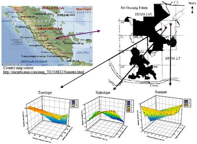 | |
| Fig. 1: | Map of study site showing the position of observation plots and the relative elevation within-plot (Note: Site map is not drawn to scale) |
Prior to computing the semivariance, spatial outliers were detected at a local scale (each topographic position within individual study sites) using the Hawkins (1980) method. This method is based on comparison among neighbourhood values and has the following formula:
| (1) |
where, zso is the spatial outlier, z(x) represents a particular data point, n is the number of neighbouring values excluding z(x), M equals the arithmetic mean of the n values and σ2 denotes the average variance for equivalently sized neighbourhoods over the sampling space.
The above equation has a chi-square (χ2) distribution with an assumption that the neighbourhood values are normally distributed. Thus, if the value calculated from Eq. 1 falls outside the expected χ2 distribution, then that z(x) is regarded as a spatial outlier.
Semivariance (γ) is estimated as follows:
 | (2) |
where, h is the separation distance between location xi or xi +h, zi or zi+h are the measured values for the regionalized variable at location xi or xi+h and n(h) is the number of pairs at any separation distance h
The process of selecting sample intervals, lag distances and semivariogram models is typically done based on trial and error. Journel and Huijbregts (1978) advocate two criteria that guide this selection process: 1) semivariograms should not include lag distances greater than about half the maximum distance between sampling points; and 2) plotted lag intervals should be short enough to allow identification of the most appropriate model to be fitted to the semivariogram.
Semivariograms were constructed for yield-influencing variable(s) from each topographic position using GS+ Version 5.1.1 (Gamma Software Design, Plainwell, MI). In constructing the semivariogram, the data were assumed to be stationary (trend-free). Stationarity of the data requires that the semivariance between any two locations in the study region depends only on the distance and direction of separation between the two locations and not their geographic location. The semivariogram was also assumed to be isotropic and omnidirectional, meaning that pairwise squared differences were averaged without regard to direction. Spatial dependence was defined using the nugget to sill ratio (Cambardella et al., 1994), which has the following interpretation:
Spatial variability information (i.e. the spatial correlation length) obtained from the semivariance analysis was used to design a suitable sampling strategy, particularly with regard to sample spacing. The minimum number of samples (nmin) required for reliable estimation of the mean value of each variable, however, was estimated using a non-spatial approach based on the following relationship (Cochran, 1977):
| (3) |
where, t is the Student function corresponding to the confidence level α, CV is the coefficient of variation and RE is the sample mean relative error (%) considered acceptable
The next stage in geo-spatial analysis was to predict values in areas that have not been sampled using inverse distance weighting (IDW) interpolation. The formula used for IDW (Isaaks and Srivastava, 1989) is:
 | (4) |
where, ![]() is the estimated value for location j, n is the number of measured data points used for interpolation, zi is the measured sample value at point i, hij represents the distance between
is the estimated value for location j, n is the number of measured data points used for interpolation, zi is the measured sample value at point i, hij represents the distance between ![]() and zi, s is the smoothing factor and p is the weighting power*
and zi, s is the smoothing factor and p is the weighting power*
Cross validation: Interpolated values were assessed for accuracy using a cross-validation procedure (Isaaks and Srivastava, 1989) based on the criteria proposed by Delhomme (1978) and Dowd (1984). Firstly, the interpolated mean error (ME) should be close to zero. The ME is calculated as follows:
| (6) |
where, n is the number of sample points ![]() , is the predicted value of the variable at point xi and x(xi) is the measured value of the variable at point xi.
, is the predicted value of the variable at point xi and x(xi) is the measured value of the variable at point xi.
Secondly, the Mean Squared Error (MSE) should be less than the sample variance. The MSE is given by:
| (7) |
Thirdly, the ratio of theoretical and calculated variance, called the standardized mean squared error (SMSE), should be approximately close to one. The SMSE is given by:
| (8) |
where, σ2 is the theoretical variance
RESULTS AND DISCUSSION
Comparison of variables across topography: A clear yield gradient existed across topographic positions in the following order: toeslope > sideslope > summit. The toeslope tested high for almost all leaf (N, P, K and Ca) and several soil variables (pH, OM, Ca). Soils at the toeslope were sandy clay in texture. In contrast, the majority of lower test values, particularly leaf N, P, Ca and soil pH, P, Ca, emanated from the summit. Soils at the summit and the sideslope were light clay in texture. Differences in soil K, Mg and ECEC were not significant across topography (Table 1).
| Table 1: | Comparison of variables (leaf and soil) and the corresponding yield across topography at Sri Gunung estate |
 | |
| 1Expressed in the following units: % (for leaf nutrients and soil OM), mg kg-1 (for soil P) and m.e. 100 g-1 (for soil K, Mg, Ca and ECEC) | |
| 2Interpreted based on International Society of Soil Sciences (ISSS) scheme (where: LC = Light clay, SC = Sandy clay) | |
| 3Reported as 3-month average FFB (kg) palm-1 | |
For each experimental site, mean values followed by the same superscript along each row are not significantly different at p = 0.05
 | |
| Fig. 2: | Semivariograms of YIVs at the toeslope |
| Table 2: | Yield influencing variables (YIVs) across topography |
 | |
| ●Developed separately using the following group as yield predictors: (1) leaf variables, (2) leaf nutrient ratios, (3) soil variables and (4) topsoil nutrient ratios | |
Yield-influencing Variables (YIVs): Regression models were developed to explain the dependence of oil palm yield on measured leaf and soil variables at each topographic position (Table 2). These production models clearly differed across topography. All three positions had significant models. Generally, both leaf and soil variables showed comparable predictability (based on R2 values).
Spatial structure assessment: Semivariograms for the toeslope YIVs (leaf N, leaf P, leaf Mg and pH) were constructed based on an active lag of 85-110 m (Fig. 2).
Leaf N and leaf P did not exhibit any definable spatial structure. Meanwhile, leaf Mg and soil pH showed definable spatial structure that was described by a spherical model. Leaf Mg and soil pH demonstrated a strong spatial dependence with 84-86% of its total variation attributed to spatial variability. Leaf Mg exhibited a short correlation length of 32 m while pH showed a moderate correlation length of 81 m.
Semivariograms for the sideslope YIVs (ECEC and subsoil Mg) were constructed based on an active lag of 120 m (Fig. 3). Only subsoil Mg showed a definable spatial structure, which was described using a spherical model.
 | |
| Fig. 3: | Semivariograms of YIVs at the sideslope |
 | |
| Fig. 4: | Semivariograms of YIVs at the summit |
The spatial dependence of subsoil Mg was moderate with 74% of its total variation explainable. Subsoil Mg exhibited a short correlation length of 58 m.
Semivariograms for the summit YIVs (leaf N, topsoil K and topsoil Mg) were constructed based on an active lag of 80 m (Fig. 4). All YIVs showed definable spatial structure, which was described using an exponential model (for leaf N) and a spherical model (for topsoil K and topsoil Mg). Leaf N exhibited strong spatial dependence with 96% of its total variation explainable. Meanwhile, topsoil K and topsoil Mg also demonstrated strong spatial dependence with 99% of their total variation explainable. The spatial correlation length of leaf N, topsoil K and topsoil Mg was short at 41 , 54 and 38 m, respectively.
Implications for sampling design: To derive a rigorous sampling protocol, it is imperative that sampling points provide accurate information about the sampled population. In classical statistics, the sample mean is assumed to provide the best estimate of the population mean. The sample mean, however, does not provide any information about spatial variability. In order to account for spatial variability, a sampling protocol should effectively consider the optimal sample size and spacing from a spatial perspective (Wollenhaupt et al., 1997).
Soil variables (with the exception of pH) generally showed a higher sample size requirement than leaf variables. Sample size requirements were typically higher at a higher confidence level (CL) corresponding to a lower relative error (RE) (Table 3). These requirements differed across topographic positions at both sites. The sampling intensity employed in this study was fairly appropriate for the majority of YIVs based on the commonly acceptable criteria of a 90% CL with a 10% RE. However, the sampling intensity for topsoil K, topsoil Mg and subsoil Mg was below such criteria. Results indicated that accurate estimates (95% CL, 10% RE) of leaf test values can be obtained from a sample size comprising 5 points. Sample size requirement varied according to leaf variable in the following order:
 |
For soil variables, reasonably accurate estimates (95% CL, 10% RE) require a sample size comprising 86 points. Sample size requirements varied according to soil variable in the following order:
 |
When spatial correlation is expected, estimation of sample size should be modified to account for the fact that spatial correlation will entail a larger sample size to estimate the population mean (Mulla and McBratney, 1999).
The Effective Range (ER) for yield-influencing variables that exhibited a definable spatial structure across topographic positions is given in Table 4. At both study sites, the ER not only varied across topographic position, but also among test variables. Sample points separated by distances greater than the ER will no longer exhibit spatial correlation (Webster, 1985).
| Table 3: | Optimal sample sizes for estimating mean values of yield-influencing variables |
 | |
| Table 4: | Effective range (ER)● of yield-influencing variable (YIVs) across topography |
 | |
| ●Derived from the semivariongram analysis (Fig. 1-3) φBased on the Flatman andYfantis (1984) prognosis | |
At this juncture, it is worth noting that the semivariogram does not provide any information for distances shorter than the minimum spacing between samples. Sampling designs that are aimed at delineating spatial structures usually feature separation distances that are less than the ER. Flatman and Yfantis (1984) recommended that samples be spaced from 0.25 to 0.5 of the ER. In this study, samples were spaced 36.4 m in the X direction (between palms) and 8.7 m in the Y direction (between rows). This spacing corresponds to 0.4-1.5 and 0.1-0.3 of the ER (computed for YIVs) in the X and Y directions, respectively. Generally, the sample spacings used in this study were fairly adequate for the soil variables but more intensive than necessary for the leaf variables. According to Webster (1985), close spacings is one way of minimizing the nugget effect. Previous research done by Goh et al. (2000) showed that the maximum spatial variation in oil palm yields from mature stands was reached within 2 to 3 palms. They attributed this to the canopy structure of oil palm, which characteristically extends to the immediate neighbouring palms only, while its roots have been shown to exploit soil resources at least 2 palms away.
 | |
| Fig. 5: | Spatial variability of (i) leaf Mg and (ii) pH at the toeslope |
 | |
| Fig. 6: | Spatial variability of subsoil Mg at the sideslope |
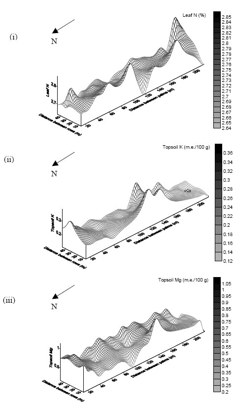 | |
| Fig. 7: | Spatial variability of (i) leaf N, (ii) topsoil K and (iii) topsoil Mg at the summit |
 | |
| Fig. 8: | Re-classed variability map of topsoil K at the summit |
| Table 5: | Cross validation of interpolated values (based on IDW) |
 | |
In practical terms, this means that any strong environmental influence on the oil palm would probably affect the nearest 3 palms most similarly. The work of Goh et al. (2000) was the only available literature to guide the choice of sample spacings for this study.
Based on a cutoff value of 70 (Mulla and McBratney, 1999), the ER data from Table 3 can be classified as narrow (Table 3) (ER less than 70 m) and moderate (ER more than 70 m). Essentially, this implies that sample spacings would depend on the type of variable being investigated and its topographic position. Using the Flatman and Yfantis (1984) prognosis, optimum sample spacings for leaf nutrients range from 8 to 18 m, while sample spacings for soil properties range from 16 to 45 m (Table 4).
Interpolation and spatial variability mapping: Interpolation was performed only on YIVs that exhibited moderate or strong spatial dependence. The distribution and pattern of both measured and interpolated values for each YIV are represented as spatial variability maps.
High values of leaf Mg were aggregated in the southern half of the plot, while high values of pH were concentrated in the north-central region of the plot. Leaf Mg was negatively correlated with pH (r = -0.73) (Fig. 5).
High values of subsoil Mg were concentrated along the North-South transect within the central region of the plot, while low values were clustered in the northeastern region of the plot (Fig. 6).
High values of leaf N were clustered along the central region of the plot in the North-South direction, while pockets of low values were evident at the western boundary (Fig. 7). Topsoil K showed a comparable distribution to that of leaf N, except that clusters of low K values were apparent in the southern region of the plot. Topsoil Mg showed a contrasting distribution of high/low values to that of leaf N. Notably, the western boundary toward the North was dominated by low Mg values. Leaf N and topsoil Mg were negatively correlated (r = -0.79).
All YIVs with the exception of subsoil Mg showed acceptable accuracy in interpolated values (Table 5). The spatial variability of these YIVs was re-mapped based on published threshold values (Foster et al., 1988; Rankine and Fairhurst, 1999). Results showed that leaf nutrients (N, P and Mg) and soil pH demonstrated moderate test values across the entire plot. Topsoil Mg was dominated by high values (99%). In contrast, topsoil K showed a distribution in the following order: 63% low values, 33.8% moderate values and 3.2% high values (Fig. 8).
Implications for management zoning: It is clear that the YIVs varied spatially across and within topographic positions. Such spatial variability can be addressed using the concept of management zones. Generally, most YIVs can be managed as a function of topography (between plots), i.e. toeslope, sideslope and summit. Evidently, yield and fertility gradients were driven by differences in topography. Considering the yield potential, application of nutrient inputs should be made in the following order:
 |
In the case of K, however, an additional level of management is appropriate based on within plot spatial variability. Higher K inputs are appropriate in the low-test areas and a standard K application rate is appropriate in the remaining areas.
CONCLUSIONS
The spatial structure of Yield-influencing Variables (YIVs) differed across topographic positions with most YIVs exhibiting moderate to strong spatial dependence that was defined by a spherical model. Variables that demonstrated a definable spatial structure showed marked differences in the sampling intensity required for reliable estimation of mean values. These variables were also subjected to varying spatial correlation lengths. Most variables showed a relatively short correlation length. Essentially, the sampling strategy in terms of size and spacing was found to depend on the type of variable being investigated and its topographic position.
A management zone concept using topography as a delineation factor seemed appropriate for the majority of YIVs. This approach would require different input rates at different topographic positions. Test values for K, however, showed clear demarcation of zones with high, moderate or low test values within plots and hence the need for variable rate application.
This study has demonstrated and quantified the spatial variability of yield-influencing soil fertility variables in small-scale plots situated at varying topographic positions. The concept of site-specific nutrient management appears to be a feasible approach to address such variability.
ACKNOWLEDGMENT
The authors are grateful to Cargill Inc. (Crop Nutrition Division and Oilseeds Division) and its plantation subsidiary (PT Hindoli, South Sumatra, Indonesia) for financial support and technical collaboration.
REFERENCES
- Cambardella, C.A., T.B. Moorman, J.M. Novak, T.B. Parkin, D.L. Karlen, R.F. Turco and A.E. Konopka, 1994. Field-scale variability of soil properties in central Iowa soils. Soil Sci. Soc. Am. J., 58: 1501-1511.
CrossRefDirect Link - Carr, P.M., G.R. Carlson, J.S. Jacobsen, G.A. Nielsen and E.O. Skogley, 1991. Farming by soil, not by fields: A strategy for increasing fertilizer profitability. J. Prod. Agric., 4: 57-61.
Direct Link - Cassel, D.K., E.J. Kamprath and F.W. Simmons, 1996. Nitrogen-sulfur relationships in corn as affected by landscape attributes and tillage. Agron. J., 88: 133-140.
Direct Link - Cochran, W.G., 1977. Sampling Techniques. 3rd Edn., John Wiley and Sons Inc., New York, ISBN-13: 978-0-471-16240-7.
Direct Link - Dowd, P.A., 1984. Cited in Paz, A., M.T. Taboada and M.J. Gomez, 1996. Spatial variability in topsoil micronutrient contents in a one-hectare cropland plot. Commun. Soil Sci. Plant Anal., 27: 479-503.
Direct Link - Flatman, G.T. and A.A. Yfantis, 1984. Geostatistical strategy for soil sampling: The survey and the census. Environ. Monit. Assess., 4: 335-349.
Direct Link - Hajrasuliha, S., N. Banniabbassi, J. Metthey and D.R. Nielsen, 1980. Spatial variability of soil sampling for salinity studies in Southwest Iran. Irrig. Sci., 1: 197-208.
CrossRefDirect Link - Russo, D. and E. Bresler, 1981. Soil hydraulic properties as stochastic processes: I. Analysis of field spatial variability. Soil Sci. Soc. Am. J., 45: 682-687.
Direct Link - Sisson, J.B. and P.J. Wierenga, 1981. Spatial variability of field-measured infiltration rate. Soil Sci. Soc. Am. J., 45: 699-704.
Direct Link - Nolan, S.C., T.W. Goddard, D.J. Heaney, D.C. Penney and R.C. McKenzie et al., 1985. Effects of fertilizer on yield at different soil landscape positions. Proceeding of the 2nd International Precision Agriculture Conference (Site Specific Management for Agricultural Systems), 1985, Madison, WI., pp: 553-558.
- Foster, H.L., A.T. Mohammed and Z.Z. Zakaria, 1988. Foliar diagnosis of oil palm in peninsular Malaysia. Proceedings of the International Oil Palm/Palm Oil Conferences-Progress and Prospects 1987-Conference 1: Agriculture, June 23-26, 1988, IPMKSM, Bangi, Selangor, pp: 249-261.
Direct Link