
Bidyut Kumar Ghosh
Dr. P.C. Mahalanabish School of Management, Supreme Knowledge Foundation Group of Institutions,Mankundu, Hooghly, West Bengal, India
Trends in Agricultural Economics
Year: 2010 | Volume: 3 | Issue: 3 | Page No.: 135-146


ABSTRACT
West Bengal is one of the agriculturally progressive states in India. The general showings of West Bengal agriculture since the eighties are impressive. Initiation of some institutional and technological changes mainly the Operation Barga and the introduction of high yielding varieties during the eighties have turned West Bengal into a progressive food grain producing state. This study attempts at studying the growth of production of some important crops as well as the variability in the crop production across the districts of the state. Using the kinked exponential methodology for growth estimation, the study reveals that the agricultural growth of major crops in West Bengal declined significantly since the mid nineties from an impressive growth rate of eighties. The decomposition of output growth of crops shows that yield growth plays the most important role behind the output growth. The contribution of the extension of area was next to yield factor. Also with the help of Kruskal-Wallis non-parametric test, the study makes it clear that the crop production variability varies significantly across the districts and, in general, the higher growth path is associated with the higher degree of variability.
PDF Abstract XML References Citation
Received: January 16, 2010;
Accepted: April 19, 2010;
Published: June 26, 2010
How to cite this article
Bidyut Kumar Ghosh, 2010. Growth and Variability in the Production of Crops in West Bengal Agriculture. Trends in Agricultural Economics, 3: 135-146.
DOI: 10.3923/tae.2010.135.146
URL: https://scialert.net/abstract/?doi=tae.2010.135.146
DOI: 10.3923/tae.2010.135.146
URL: https://scialert.net/abstract/?doi=tae.2010.135.146
INTRODUCTION
West Bengal’s economic history over the last three decades has been a mix of the good and bad. Growth rates have increased and per capita incomes have gone up. Liberalization and deregulation have yielded impressive results and the economy is increasingly integrated to the world economy. However, agriculture continues to be the backbone of the economy of the state of West Bengal. Agriculture remains the most crucial sector of the state economy as around 72% of the total population lives in rural areas and agricultural continues to be their mainstay. However, along with the structural transformation of the economy of the state, the contribution of agriculture in State Domestic Product (SDP) is observed to follow a declining trend. Though the contributions of agriculture to total SDP at constant prices has declined from 41.16% in 1970-71 to 27.1% in 2000-01, it contributes a significant share to the SDP as compared to other sectors of the economy. West Bengal is one of the states of the country where the expansion of Net Cropped Area (NCA) has almost reached a point of saturation. The data on land utilization pattern published by Bureau of Applied Economic and Statistics shows that Net Cropped Area in the state has registered a marginal fall of 1.05% during the period 1995-96 to 2000-01. The cropping intensity of the state has also shown a sign of stagnancy. In 2000-01, it was 168% (i.e., an increase of only 2.44% compared to 1995-96). In 2003-04, it was 178%.
Foodgrain dominates the cropping pattern of the state (De, 2002; Ghosh and Kuri, 2005). Food grain crops are grouped as cereals crops and pulse crops. The important cereals crops of the state include rice, wheat and maize. On the other hand, pulses include mainly gram, arhar, muskalai (urad), masur (lentil), khesari etc. The state also produces some important cash crops like jute, potato etc. In 2000-01, food grain crops including cereals and pulses occupied 68 pert cent of Gross Cropped Area. With the production of 16501.24 thousand tones, West Bengal occupied the top position in the food grain production in India. Though the state performed well in foodgrain production among the states of India, in recent years there is evidence of the stagnancy in foodgrain production growth rate (Ghosh and Kuri, 2007). Further, the expansion of area under cultivation is hardly possible in West Bengal. Productivity growths of most of the important crops were stagnated in the 1990s after the liberalization process began. The growth performance of the state has been analyzed by many researchers (Saha and Swaminathan, 1994; Boyce, 1987; Chattopadhyay and Das, 2000). However, most of studies belong to the period of eighties or early nineties. Not too many works are done on the issue of growth of agriculture especially after the implementation of liberalisation policy. Under this backdrop this paper deals with the renewed enquiry into the time series analysis of the crop production for the period 1970-71 to 2004-05. The specific objectives of this study are:
| • | To measure the growth rates of the major crops in West Bengal during different sub-periods under study |
| • | To examine the acceleration or deceleration in the growth performance of major crops |
| • | To measure and examine the level of variability in total agricultural output and in the production of major crops. |
MATERIALS AND METHODS
The study is extended for the time period extending from 1970-71 to 2004-05 and it is based exclusively on the secondary data collected from the Statistical Abstracts (1974-75, 1980-81, 1984-85, 1990-91, 1995-96, 2000-01, 2003-04) of West Bengal published by the Bureau of Applied Economics and Statistics, Government of West Bengal (henceforth bureau). District Statistical Handbook is another publication of the Bureau that contains database for each district.
For measuring agricultural growth rate, linear trend equation:
| (1) |
where, Qt is the output at period t, t is the time is used. In this equation b gives us an estimate of the absolute increase of agricultural output per unit of time, a the constant appearing in the regression line and ut the error term in the regression line. However, for measuring the acceleration or deceleration in the growth rate the log quadratic trend equation:
| (2) |
is fitted to examine the acceleration (or deceleration) in the growth trend. A positive significant value of c indicates acceleration while a negative implies a deceleration.
To measure the growth rates in different sub-periods the following kinked exponential model is used :
| (3) |
In this equation b1, b2 and b3 are the growth rates for the first, second and third sub-periods respectively. Estimating the trend break equation also tests the significance of the difference between the growth rates in two different sub periods:
| (4) |
where, b1* and b2* are the difference between the first and second sub-period growth rates and the difference between the third and second sub-period, respectively.
Coefficient of Variation (CV) has been used to measure the variations in production of crops. There may be variation in the production of crops over the years. Also there are chances that the crop production may vary across the different districts of the state. In this study we have measured the variability in the production of important crops over the three distinct sub-periods across the districts of the state. The difference in CVs of the three distinct periods is tested by Kruskal-Wallis test (Anderson et al., 2008). The hypothesis for the Kruskal-Wallis test can be written as follows:
| • | H0: Sub-period CVs are identical |
| • | H1: Sub-period CVs are not identical |
The Kruskal-Wallis test statistic, which is based on the on the sum of ranks for CVs of each of the districts during the three different sub-periods for any particular crop can be computed as follows:
Kruskal-Wallis test statistic
| (5) |
Where:
| k | = | The number of population (here sub-periods) |
| ni | = | The number of observation in the sample i |
| nt | = | Σni = Total umber observation in all sample |
| Ri | = | Dum of ranks for sample i |
Under the null hypothesis in which the populations are identical, the sampling distribution of W is approximated by a Chi-square distribution with k-1 degrees of freedom.
RESULTS AND DISCUSSION
Sub-Period Growth Rates: Kinked Exponential Method
The pioneer work came from Boyce (1987) who measured the growth rates of crop output in West Bengal agriculture during 1949-80. He observed that the stagnancy of agriculture of the state comes to an end during 1980s and the growth of agricultural rose to its highest level during the decade of eighties. Saha and Swaminathan (1994) estimated growth of aggregate crop output of 6.40% during the eighties was the highest among the Indian states and this spectacular growth of the agricultural sector was widespread in the districts of the state. They argue that the land reforms measures introduced in the state during the early 1980s have significantly contributed to the impressive growth of the agriculture of the state. Chattopadhyay and Das (2000) also claim that the agricultural growth in West Bengal during eighties is higher than the seventies. However, their estimate of the annual growth rate of agricultural production (3.6%) in West Bengal during 1977-78 to 1994-95 is much lower than that (6.4%) estimated by Saha and Swaminathan (1994) during the period 1981-92 to 1990-91. They conclude that agricultural production in West Bengal is still dependent on rainfall and fluctuations in rainfall index significantly positively contribute to the fluctuations in agricultural production in the state. Sanyal et al. (1998) and Mukherji and Mukhopadhyay (1995) also support the view of Saha and Swaminathan (1994) that land reforms programmes is primarily responsible for the breakthrough in West Bengal agriculture. Harris (1992), however, believes that this high growth has taken place in the absence of any reform of the agrarian structure. In his opinion, this was rather technological-'suitable technology' coined with favourable fertilizer-paddy price ratio. To analyze the performance of agricultural sector of the state the main emphasis has been given on the decadal growth rates of the major crops. We measure the sub-period growth rates of area, production and yield of the crops as measured by the kinked exponential growth model. For convenience, the whole period of 35 years (1970-71 to 2004-05) is divided into three sub-periods; first sub-period (1970-71 to 1980-81), second sub-period (1981-82 to 1991-92) and third sub-period (1992-93 to 2004-05). These three sub-periods have special significance to the economy of West Bengal. Clearly, the agricultural development of the state during the period 1970-71 to 1980-81 was not up to the mark, rather it was underdeveloped in nature. However, some institutional and technological changes took place in the state during the early 80s. This institutinal and technological changes had some positive impact on the agricultural development of the state. The productivity and production of all important crops have increased significantly. Lastly, the third sub-period (1992-93 to 2004-05) is the period of LPG (liberalisation, privatisation and globalisation). Clearly, the final sub-period captures the impact of globalisation on the agriculture of the state.
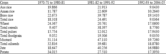
During the first sub-period (1970-71 to 1980-81) it has been observed that the growth rates of production of almost all important crops were either low or even negative. For example, total rice grew only at 0.51% per annum. The output growth rates of all the three varieties of rice were also very low during the 70s. The growth rates of production of Aman, Aus and Boro were 0.52, -4.32 and 2.53% per annum, respectively. The growth rates of production of wheat (-3.18% p. a.), total cereals (-3.23% p.a), jute (-1.74% p.a) and total pulses (-3.16% p.a.) were negative during this period (Table 1). Simple decomposition of output into area and yield indicates that neither area nor yield growth rates were impressive. In most cases, the area and yield growth rates (Table 2, 3) were either very slow or even negative, which in turn forces the output growth rate to be negative. The output of crops such as potato, mustard and total oilseeds were, however, positive during the decade of seventies. For potato, the high growth of area under cultivation was the main thrust behind the output growth rate as around 66% of the production growth came from area expansion and the remaining 34% came from yield growth rate. In case of mustard, the yield growth explains 65% of the output growth rate and the remaining 35% has been contributed by the area expansion. For the total oilseeds, the area expansion explains the majority of the output growth rates. Total foodgrain production which is the sum of total cereals and total pulses grew at a nominal growth rate of only 0.35% per annum with a negative area growth rate of 0.51% per annum.
| Table 1: | Sub-period growth rates of production of crops in West Bengal during 1970-71 to 2004-05 |
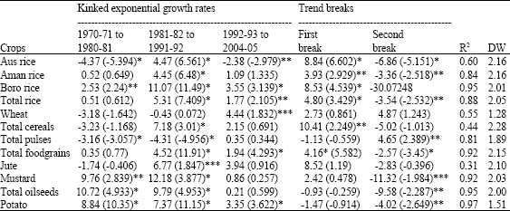 | |
| Source: Author’s calculation based on BAES data. *p = 0.01, **p = 0.05, ***p = 0.1 | |
| Table 2: | Sub-period Growth rates of area under crops in West Bengal during 1970-71 to 2004-05 |
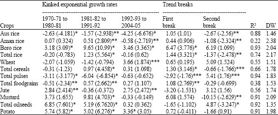 | |
| Source: Author’s calculation based on BAES data. *p = 0.01, **p = 0.05, ***p = 0.1 | |
| Table 3: | Sub-period Growth rates of yield of crops in West Bengal during 1970-71 to 2004-05 |
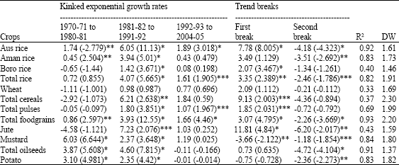 | |
| Source: Author’s calculation based on BAES data. *p = 0.01, **p = 0.05, ***p = 0.1 | |
In fact, a positive yield growth rate (0.86%) resulted the food production to grow at a slow positive growth rate. As already mentioned that the jute production grew at a negative rate during the decade of 70s and this negative production of growth was mainly due to the yield growth of jute which was estimated to be -4.58% per annum.
Thus, we find that during the period 1970-71 to 1980-81, without few exceptions the growth rates of production of most of the crops were slow. Both the area expansion under crops and the yield of the crops were responsible for this slow growth of output. This situation of slow growth, however, changed during the 80s when the growth rates of area, production and yield of all the crops improved significantly. From Table 1, it is found that during the second sub-period (1981-82 to 1991-92), the output growth rates of total rice improved significantly from a negative growth rate observed during the previous decades of 70s to 1.23% per annum during the second sub-period and this increment in growth rate was significant (as tested by the significance of trend breaks). The factor behind the massive increment in the output growth rates of most of the major crops during the eighties in West Bengal was the improvement in the yield growth rates. The yield growth rate of total rice jumped from 0.72% per annum during seventies to 4.07% per annum during the period 1981-82 to 1991-92 (Table 3). During the second sub-period, more than 70% of the output growth came from yield growth. The similar fashion of growth trend has been observed for Aman rice. For Aus rice the growth rate of area was negative (-1.57% p. a) during the second sub-period (Table 2). However, a massive increase in the yield growth rate (6.05%) during the 80s resulted in the impressive growth of output at a rate of 4.47% per annum. In case of Boro paddy quite an opposite scenario has been observed where the area growth rate plays the major role behind its impressive output growth of over 11% per annum during the second sub-period. Boro was introduced on massive scale as HYV crops in the state during the early 80s. As it was a HYV crop, its yield level was already high and its high yield was the main factor for its rapid expansion in the state. As far as wheat is concerned, it is found that the state has been able to achieve a marginal positive growth rate as against the negative growth of the 70s. However, during this period the performance of the state in respect of pulse production was very gloomy. The negative growth rate of the 70s became much more acute during the eighties. However, the impressive growth performance of paddy crops has turned the growth of foodgrain production to an optimum level of 4.52% per annum during the second sub-period. This was one of the best foodgrain production performances among the states of Indian union. The sluggish growth of pulse crops did not affect the overall foodgrain production because the share of pulse crops to the total foodgrain both in terms of area and production was small compared to total cereals. This impressive growth performance has also been observed for the crops such as mustard, Til, total oilseeds, jute and potato. During the period of eighties, the growth of production of all these crops was very much higher compared to the previous period and, in general, the yield growth rate played the most dominant role behind their impressive growth performance during eighties. The production growth rate of mustard jumped from 9.76% during the first sub-period to 12.18% during the second sub-period with more than 80% contribution coming from the expansion of area under mustard crops. The same is true for the total oilseeds.
However, the state failed to sustain the high growth path as achieved during the eighties. The growth rate of production of almost all important crops declined in the subsequent periods. The area growth rate of Aman rice becomes negative during the decade of nineties and the yield growth rate also reduced significantly. As a result of which the output of Aman rice declined only to 1.05% per annum. During the nineties, the output growth rate of Boro rice declined to 3.35% per annum and this fall in growth rate is significant (Table 1). Considering all the cereals crops together, it is found that due to the significant fall in yield rate, the output of total cereals declined drastically to 2.15% per annum during the third sub-period from 7.18% per annum during the second sub-period. The same is the case for total foodgrain. The state experienced a very high growth rate of production of mustard during the eighties. However, the state has not been able to sustain the tempo of high mustard production growth for a very long period. The mustard production growth rate declined very drastically to only 0.86% per annum during the third sub-period of 1992-93 to 2004-05. For total oilseeds, the yield plays the dominant role behind output growth rate during the eighties and the drastic fall in yield rate (4.60% per annum during 80s to -0.11% per annum during 90s) forced the output to grow at the rate of 0.21% per annum only.
For another important cash crop potato, the performance during nineties was not as good as observed during the previous sub-periods. The output growth rates for potato was 8.84, 7.37 and 3.35%, respectively in the first, second and third sub-periods respectively (Table 1). And the difference in the growth rate between the third (1992-93 to 2004-05) and second sub-period (1981-82 to 1991-92) was significant at 5% level of significance. From the Table 1-3, it is clear that the main reason for this decline in output growth rate is the slowing down of the yield growth rate, which reduced to -0.01% per annum during the period 1992-93 to 2004-05 from 2.35% per annum during the previous sub-period (1981-82 to 1991-92).
Thus, we see that the performance of the agricultural sector in the state of West Bengal during the period of eighties in terms of growth rates of production of important crops is better than that of during seventies and nineties. The expansion of area under cultivation of major crops almost reached a level of saturation. The growth rates of yield of major crops have decreased to a significant level and this the fall in the yield growth rates of the major crops reduces the growth of production of the major crops.
Acceleration and Deceleration in Trend Rates of Growth
To examine the acceleration and deceleration in growth rates of production of some important crops in West Bengal, the log-quadratic trend equation is fitted to the data and the results is shown in the Table 4. The results show that during the period 1970-71 to 1980-81, there were marked decelerations in the growth trend of almost all major crops of the state. However, during the period of eighties the growth trend of crops such as aman and aus rice, total rice, total foodgrain and jute experienced positive acceleration in their growth rates. Total pulse production of the state which experienced deceleration in growth trend during the first two sub-periods registered acceleration in growth in the final sub-period of nineties. During the nineties potato, jute, wheat and boro rice registered significant deceleration in their growth trend. It is to be noted that wheat is a crops which experienced deceleration in growth trend in all the sub-periods. Thus, in general, there seems to be decelerating trend in the growth of major crops in West Bengal since nineties.
| Table 4: | Growth and acceleration in crop output in West Bengal using Log Quadratic form, 1970-71 to 2003-04 |
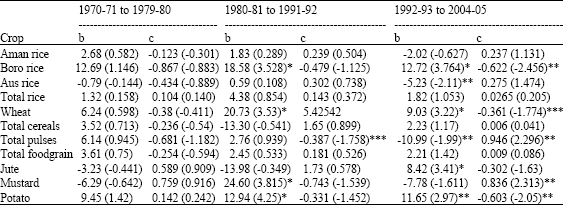 | |
| Source: Author’s calculation based on BAES data. *p = 0.01, **p = 0.05, ***p = 0.1 | |
| Table 5: | Coefficient of variation of production of major crops in West Bengal |
 | |
Variability of Production of Major Crops
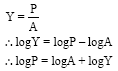
Using the coefficient of Variation (CV) the variability of production of major crops in West Bengal during 1970-71 to 2004-05 has been examined. An attempt has also been made to examine the contribution of area, yield variability in the variability of the total production of the selected crops separately for three periods viz. 1970-71 to 1980-81, 1981-82 to 1991-92 and 1992-93 to 2004-05. Further, the difference in coefficient of variation values of three sub-periods based on the districts of the state for each crop was tested by Kruksal-Wallis rank test.
The variability of production of major crops is reported in Table 5. By looking at the production variability of crops as measured by the coefficient of variation at the state level the following important outcomes emerge:
| • | For total rice, the highest variability was found in the second sub-period. It is interesting to note that during the second sub-period the highest variability in production is associated with the highest rate of growth of production. The least variability was found in the third sub-period where production growth rate was also found the least among the three sub-periods. Thus for total rice , it can be said that the period of highest growth coincided with the period of highest variability in production |
| • | For wheat and total pulse production almost equal level of variability in production has been observed across the three sub-periods |
| • | The state shows a high degree of variability in the second sub-period as compared to the other two sub-periods in respect of rice (including its three varieties), total foodgrain, mustard, total oilseeds and jute |
| • | For the two cash crops the state was found to have a higher degree of variability in the jute production in the second sub-period. The other two sub-periods show equal and moderate level of variability. For the potato crop the variability was found to decline continuously in all the sub-periods |
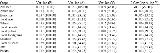
Decomposition of Production Variability
To examine the contributions of area, yield and their interactions effects on the variability of total production, we use the following decomposition scheme.
We know:
 |
| Table 6: | The decomposition of output variability into its various components during 1970-71 to 1980-81 |
 | |
| Source: Author’s calculation based on BAES data | |
| Table 7: | The decomposition of output variability into its various components during 1981-82 to 1991-92 |
 | |
| Source: Author’s calculation based on BAES data | |
| Table 8: | The decomposition of output variability into its various components during 1992-93 to 2004-05 |
 | |
| Source: Author’s calculation based on BAES data | |
Where:
| P | = | Production |
| A | = | Area |
| Y | = | Yield |
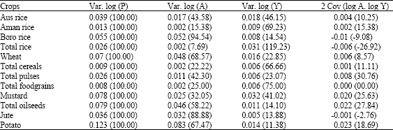
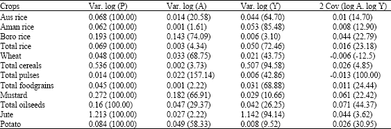
The decomposition of production variability in to its different components is done for the three sub-periods for each of the crops and the results are shown in Table 6-8. The major outcomes of this production variability decomposition are outlined as follows:
| • | For the total rice, the yield variability was found to be the single most important factor behind the production variability in all the sub-periods. The contribution of area and interaction of area and yield were never been important factors in the output variability. Among the three varieties of rice, for aus rice during the first and second sub-periods both area and yield variability play almost equal role in explaining the production variability and their interaction did not cause any serious effect on production variability. However, the effect of yield variability on total production variability increases during the second sub-period. During the third sub-period, the output variation was highly influenced by the fluctuations in area under aus cultivation and also the interaction effect became negative. For boro rice, in all the sub-periods, the fluctuation in area under cultivation was the main factor of output variation in the state of West Bengal. Like total rice, in the total cereals and in total foodgrains production, fluctuations in yield/or productivity variability is mainly responsible for output variability. The area and interaction factors hardly play any role during the second sub-period |
| • | In case of total pulse, the variability of area contributes the largest percentage share of the output variability in all the sub-periods. In the second sub-period, it has been found that the area variability was more than 150% of the output variability and the interaction effect was also high and negative. However, in the third sub-period the areas under pulse crops tend to increase steadily and output variability was caused almost equally by area and yield variability. Also 29.03% of the output variability came in the form of interaction of area and yield fluctuations |
| • | During the first sub-period, the fluctuation in the area under cultivation causes the maximum variation in total oilseed output fluctuation. However, during the next two sub-periods, the area under oilseeds cultivation expanded steadily and all three components of output variation play almost equal role in explaining the production variability of total oilseeds |
| • | Among two important cash crops of the farmers of the state, the variability of area under cultivation of potato is the main factor behind the output variability during the all sub-periods. For jute crop, two complete different scenarios were found the first and second sub-periods. During the first sub-period, the changes in the area under cultivation causes as much as 88% of the total output variability and the yield factor explains only 13% of output variability. The interaction effect was negative; however, it is very small. In the next sub-period the variability in the yield explains more than 90% of production variability |
| • | Final sub-period all the three components of output variability explained the significant variation in the variability of production of jute in the state. On the hand, the variation in the area under cultivation always remained the most important factor of potato production variation in all the sub-periods in West Bengal |
Test of Difference in the Variability of Crop Output: Kruksal-Wallis Test
The significance of the difference in C.V values of three sub-periods based on the fifteen districts for each crop was tested by Kruksal-Wallis test. The results are displayed in Table 9. The result indicates that there was no significant difference in the variability of production of total pulse among the sub-periods. However, it was observed that the sum of ranks for period III and period II were almost equal and much higher than that for the period I, implying that variability in total pulse production was less in the 70s as compared to the 80s and 90s. For all other crops, except aus rice, the K-W test statistic was found to be significant, implying that the crop production variability differ significantly in all the three sub-periods.
| Table 9: | Estimated Kruskal-Wallis test for variability in West Bengal agriculture |
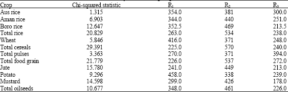 | |
| Source: Author’s calculation based on BAES data. R1 = Sum of ranks in period I (1970-71 to 1980-81); R2 = Sum of ranks in period II (1981-82 to 1991-92); R3 = Sum of ranks in period III (1992-93 to 2004-05) | |
Furthermore, because the CV ratings are higher in the second sub-period for the crop jute, total cereals, total food grain and total rice, it can be said that the high growth rate of 80s was associated with high degree of variability. For wheat and potato the period of 70s was found to have highest variability in production. In the decade of 90s the variability of production was found to be stabilized for all crops. During this decade the growth rates of production of all major crops were also found to stable and reached a saturated level.
Thus, in short it can be said that except Aus rice and total pulses, there is significant variation in the production of all other crops across the districts in all the three sub-periods. The high growth path of the decade of eighties, in general, is associated with the high degree of variability. However, the variation was found to be stabilized during the decade of nineties.
CONCLUSIONS
The study makes it clear that the agriculture of the state had been able to boost its performance during the decade of eighties, at least in terms of growth rates production of major crops, mainly for tremendous increment in the yield growth rates of the crops along with expansion of area under cultivation. The effective introduction of HYV technology coupled with successful implementation of land reforms programme at the very grass root level set the path of agricultural development in the state of West Bengal. However, this scenario of impressive growth performance did not sustain for a very long period of time. The fall in the yield growth rates of crops reduces the production growth rates during the era of globalisation which have been started in the early nineties. During this period, crops such as Boro rice, total foodgrain, mustard, jute, potato experienced fall in their growth rates to a significant extent with marked deceleration in growth trend. Again so far as variability of crop production is concerned it can be concluded that the higher growth path is associated with the high degree of production variation across the districts of the state during eighties. The degree of variation was found to be stabilized during the nineties. The decomposition of variability clearly reveals that yield variability of crops, in general, is the prime factor behind crop production variability.
The cultivation of the same crop on the same piece of land over a long period and non-optimum doses of chemical fertilizer might cause the soil fertility to decline in the state. This is also very much prominent from the stagnation of yield level of most the important crops in West Bengal in the recent years. And this stagnation or slowing down of yield growth rates of major crops cause the total agricultural output to grow at a slower rate in the recent times. This is the main cause of concern of today, especially with respect to the food security issue of the state.
REFERENCES
- Chattopadhyay, A.K and P.S. Das, 2000. Estimation of growth rate: A critical analysis with reference to West Bengal agriculture. Indian J. Agric. Econ., 55: 116-135.
Direct Link - Ghosh, B.K. and P.K. Kuri, 2007. Agricultural growth in West Bengal from 1970-71 to 2003-04: A decomposition analysis. ICFAI J. Agric. Econ., 4: 30-46.
Direct Link - Saha, A. and M. Swaminathan, 1994. Agricultural growth in West Bengal in the 1980s: A disaggregation by districts and crops. Econ. Political Weekly, 29: A-8-A-8.
Direct Link - Sanyal, M.K., P.K. Biswas and S. Bardhan, 1998. Institutional change and output growth in west Bengal agriculture: End of impasse. Econ. Political Weekly, 33: 2979-2986.
Direct Link - Harris, J., 1992. What is happening in rural West Bengal: Agrarian reforms, growth and distribution. Econ. Political Weekly, 28: 1237-1247.
Direct Link - Mukherji, B. and S. Mukhopadhyay, 1995. Impact of institutional change on productivity in a small-farm economy: Case of Rural West Bengal. Econ. Political Weekly, 30: 2134-2137.
Direct Link