
Faisal G. Khamis
College of Business Administration, Al-Ain University of Science and Technology, United Arab Emiarat
Trends in Applied Sciences Research
Year: 2014 | Volume: 9 | Issue: 7 | Page No.: 345-359


ABSTRACT
Reducing mortality inequalities is a global priority. Geographic mortality inequalities have been widely discussed in most of the developed and a few developing countries, with poorer areas experiencing poorer health and higher mortality risks than richer areas. Spatial analysis is a relevant set of tools for studying the geographical distribution of mortality. This study aimed to investigate the spatial structure of children mortality across Egypt’s governorates. The study design is a cross-sectional analysis using census data collected in 2007. Three indicators of Mortality Factor (MF) were studied: Newly Born Mortality Rate (NBMR), Infant Mortality Rate (IMR) and below five years Children Mortality Rate (CMR). Data were analyzed using descriptive statistics and mixed methods approach: Factor analysis, spatial statistics and mapping to address two questions: (1) Does spatial clustering of MF exists in Egypt? and (2) If so, what is the number of such clusters and their locations? Global Moran’s I-statistic for MF was found to be 0.15 with z = 1.76, p = 0.79 and permutation p = 0.068. Local Moran’s Ii for four significant clusters were found as follows: I2 = 0.70, p = 0.30; I11 = 0.99, p = 0.028; I12 = 0.87, p = 0.008 and I22 = 0.84, p = 0.026. The study concludes that the spatial pattern of MF is concentrated in the northern and middle governorates based on visual inspection. Global clustering of MF was not found significant, but four significant local clusters were found in the northern and southern governorates based on local Moran statistic. These conclusions illustrate the importance of identifying the governorates which have higher children mortality rates that have implications for social policy and public health interventions.
PDF Abstract XML References Citation
Received: February 28, 2014;
Accepted: April 26, 2014;
Published: June 05, 2014
How to cite this article
Faisal G. Khamis, 2014. Exploring Children Mortality in Egypt-2007 using Factor Analysis, Spatial
Statistics and Mapping. Trends in Applied Sciences Research, 9: 345-359.
URL: https://scialert.net/abstract/?doi=tasr.2014.345.359
URL: https://scialert.net/abstract/?doi=tasr.2014.345.359
INTRODUCTION
The children mortality is a major public health problem in some developed and most developing countries. Obviously mortality is a regressive social phenomenon that continues to plague developing countries and thus, requires a considerable attention. The arisen question is whether the spatial pattern of children mortality was existed in Egypt in 2007? The importance of studying the mortality is issued from the statement by Navaneetham et al. (2008) stated that mortality levels and patterns can lead to increases in poverty and/or hunger. Navaneetham et al. (2008) stated the rural population in north India was suffered in both spatial patterns in infant mortality and generalized deprivation.
To understand the spatial pattern of mortality, the investigation should focus on the features of areas rather than on compositional characteristics of residents of the area which cannot fully describe the social environment in which people live (Macintyre et al., 1993). In recent years, a growing interest has been seen in examining the existence of spatial autocorrelation in mortality. However, governorates are tightly linked by migration, commuting and inter-governorate trade. These types of spatial interaction are exposed to frictional effects of distance, possibly causing the spatial dependence of governorate conditions.
As everyone knows children mortality was studied in many countries. For example, Adair (2004) presented analysis for the spatial distribution of Children Mortality Rate (CMR) in the Indonesia’s sub-districts within Jabotabek, Bandung and Surabaya. Adair’s study results showed large differences in CMR within these regions. He stated that the large discrepancies in socio-economic status within these mega-urban regions will affect the relative risk of child mortality within the population. This condition has existed in several countries. For instance, Luginaah et al. (2001) investigated the characterization of neighbourhoods based on socioeconomic determinants of health correspond spatially with mortality patterns in Hamilton, Ontario, Canada. Luginaah et al. (2001) used approximately the same mixed-methods approach, census tracts were used as the smallest geographic units that the author used in this study (census governorates were used). Luginaah et al. (2001) study suggested the existence of at least four neighbourhoods with characteristics likely to be associated with health status. The UN-Habitat 2010-2011 report on the state of the world’s cities identified the spatial isolation of poor people in cities as one of the major challenges in developing countries. As people and cities in the developing world get richer, the worry is that the spatial socioeconomic segregation of poor people increases which in turn may increase their risks of mortality and poor health. Rich wards surrounded by poor areas have higher coronary heart disease mortality rates than rich wards surrounded by rich areas and vice versa (Allender et al., 2012). Auger et al. (2012) stated income inequality is associated with mortality in Canadian-born individuals but not immigrants.
De Pedro-Cuesta et al. (2009) identified some clustered municipalities with high mortality in Spain were situated near industrial plants reported to be associated with environmental xenobiotic emissions. Gupta (1990) stated the risk of dying in Rural Punjab, India was distributed very unevenly amongst children, as the majority of child deaths were clustered amongst a small proportion of the families. Gupta concluded the death-clustering variable remained significant even after several possible biological and socioeconomic reasons for clustering had been controlled. Several statistically significant clusters of higher childhood mortality rates comprising different sets of villages were identified in sub-Saharan Africa by Sankoh et al. (2001). A statistically significant spatial heterogeneity of a very small magnitude was observed by Bellec et al. (2006) in the incidence of childhood acute leukaemia in the whole French territory over 1990-1994.
Understanding the distribution of children mortality in space is important for identifying communities at high risk. Reducing mortality inequality especially in children is not a primary objective but emergent prosperity. The importance of the research goal or purpose was followed from such argument stated that mortality is a standard indicator for health status of the population. To author’s knowledge no studies used mixed methods approach: Factor analysis, spatial analysis and geographical mapping in studying the mortality inequality in Egypt. Very limited studies regarding the children mortality were conducted in Egypt. That’s why, the author reviewed several studies regarding children mortality clustering conducted in several developing and developed countries.
The importance of mapping was stated by Koch (2005), why make the map if detailed statistical tables carry the same results? Maps provide a powerful means to communicate data to others. Unlike information displayed in graphs, tables and charts, maps also provide bookmarks for memories. They remind us of places we visited, a childhood home and locations of historical events. In this way, maps are not passive mechanism for presenting information. As a result, choropleth map is quite commonly used in public health studies, at least for descriptive statistics, before more in depth analysis is carried out. Perhaps the most important reason for studying the spatial statistics is not only the interest in answering the “how much” question, but the “how much is where” question (Schabenberger and Gotway, 2005). In light of these (1) The existence of spatial global clustering, (2) Spatial local clusters of governorates in children mortality were investigated and (3) Mapping was applied for mortality factor and its local Moran’s Ii values.
The study design is a cross-sectional analysis in a census survey conducted in Egypt in 2007. In conclusion, the spatial global clustering was not found, but several local clusters in mortality were found in the northern and southern governorates. The major contribution in the present study is the demonstration that the spatial locations have statistically significant effects on the likelihood and the disparity of children mortality in Egypt.
MATERIALS AND METHODS
Data: Data were collected from the book of Egypt’s description by information in 2009, based on census conducted in Egypt in 2007. For each of (N = 27) governorates, three indicators (observed variables), NBMR, IMR and below 5 years CMR were studied. The NBMR is the mortality rate of infants below 28 days of age per 1000 live births. The IMR is the mortality rate of children below one year old per 1000 live births. Below 5 years CMR is the mortality rate of children under five years old per 1000 live births. In Egypt, the NBMR, IMR and below 5 years CMR decreased slightly-moderately from 10.3, 26.4 and 33.8, respectively in 2000 to 8.4, 19.2 and 24.3, respectively in 2007.
Analysis: This study employed mixed-methods approach to study the children mortality pattern. Data analysis involved seven steps:
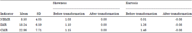
| Step 1: | The three indicators, NBMR, IMR and below 5 years CMR were tested for normal distribution. They were not found to follow normal distribution. Therefore, all indicators were transformed to normal distribution using LISREL software. LISREL scales normal scores so that transformed variable has the same sample mean and standard deviation as the original variable. Thus, normal score is a monotonic transformation of original score (this characteristic can be considered as an advantage in this transformation) but with values of skewness and kurtosis much reduced |
| Step 2: | Factor analysis was applied to create the children Mortality Factor (MF), unobserved variable (or observed indirectly) |
| Step 3: | Visual inspection was conducted based on quantified gradients of MF using quartiles |
| Step 4: | Included the calculation of global Moran’s I-statistic for MF to detect the global clustering. Then, the significance of I-statistic was examined using permutation test |
| Step 5: | Involved the calculation of local Moran’s Ii for ith governorate to detect the local clusters for MF |
| Step 6: | Included the calculation of p-value of local Moran’s Ii using Monte Carlo simulation |
| Step 7: | Using quartiles, visual inspection for the gradients of local Moran values was inspected based on choropleth mapping |
Factor analysis: Factor analysis is a technique often used to detect and assess latent sources of variation and covariation in observed measurements. For a given set of response variables one wants to find a set of underlying latent factors, fewer in number than the observed variables. Regression method was used to estimate children MF scores that explain much of the variance observed from the original variables. The following factor model with respect to this study can be explained as follows:
y(3x1) = Λ(3x1)η+ε(3x1)
where, y’ = (y1, y2, y3) was measured in deviation from the mean of transformed NBMR = y1, IMR = y2 and below 5 years CMR = y3, respectively. The η is the unobservable MF required to be estimated. The Λ is the matrix of factor loadings. The ε is the matrix of errors.
Factor analysis with a Maximum Likelihood (ML) approach (Johnson and Wichern, 2002) was employed to identify the MF. The MF score was computed for each governorate using regression method as follows:
where, ![]() is the estimated MF score for jth governorate,
is the estimated MF score for jth governorate, ![]() is the ML estimates of the factor loadings, S(3x3) is the sample covariance matrix, yj is the (3x1) vector of three indicators of MF.
is the ML estimates of the factor loadings, S(3x3) is the sample covariance matrix, yj is the (3x1) vector of three indicators of MF.
Cronbach’s alpha is commonly used measure of reliability (internal coherence) for a set of two or more construct indicators. Cronbach’s alpha for MF was found 0.91 which indicates a high level of internal consistency (reliability coefficient of 0.70 or higher is considered acceptable in most social science research situations). The MF obtained was categorized into quantiles of four intervals, to be used for choropleth mapping. Such approach enables qualitative evaluation of spatial pattern of mortality and gives visual inspection only. A children MF was used in the next step of spatial analysis.
Mapping: The picture equals more than 1000 words. To construct a choropleth map, data for enumeration governorates are typically grouped into classes and a gray tone was assigned to each class. The MF was categorized into four intervals using darker shades of gray to indicate increasing values. Such approach enables qualitative evaluation of spatial pattern. In the neighbourhood researches, neighbours may be defined as governorates which border each other or within a certain distance of each other. In this research neighbouring structure was defined as governorates which share a boundary. The second-order method (queen pattern) which included both the first-order neighbours (rook pattern) and those diagonally linked (bishop pattern) was used. A neighbourhood system of Egypt’s governorates is explained in Fig. 1, where ID neighbours for each governorate are shown.
Although, maps allow visual assessment for spatial pattern, they have two important limitations: Their interpretation varies from person to person and there is the possibility that a perceived pattern is actually the result of randomness and thus not meaningful. For these reasons, it makes sense to compute a numerical measure of spatial pattern which can be accomplished using spatial autocorrelation.
Spatial analysis: The goal of a global index of spatial autocorrelation is to summarize the degree to which similar observations tend to occur near to each other in geographic space. The spatial autocorrelation was tested using standard normal deviate (z-statistic) of Moran’s I under normal distribution assumption.
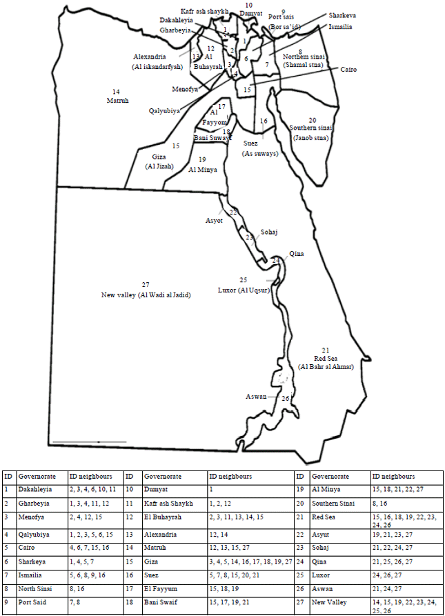 | |
| Fig. 1: | Study area shows all governorates with its ID and ID neighbours of each governorate |
Moran’s I is a coefficient used to measure the strength of spatial autocorrelation in regional data. The null hypothesis of no spatial autocorrelation or spatially independent versus the alternative of positive spatial autocorrelation is as follows:
H0: No clustering exists (no spatial autocorrelation)
H1: Clustering exists (positive spatial autocorrelation)
Moran’s I is calculated as follows (Cliff and Ord, 1981):
 |
where, N = 27 is the number of governorates, the wij = 1 is a weight denoting the strength of the connection between two governorates i and j, otherwise, wij = zero and the xi and xj represents MF in the ith and jth governorate, respectively.
A significant positive value of Moran’s I indicates positive spatial autocorrelation, showing the overall pattern for the governorates having a high/low level of the MF similar to their neighbouring governorates. A significant negative value indicates negative spatial autocorrelation, showing the governorates having a high/low level of the MF unlike neighbouring governorates. To test the significance of global Moran’s I, z-statistic that follows a standard normal distribution was applied. It is calculated as follows (Weeks, 1992):
Permutation test was applied. A permutation test is used to know a certain pattern in data is or is not likely to have arisen by chance. The scores of the MF was randomly reallocated 1,000 times with 1,000 of spatial autocorrelations were calculated in each time to test the null hypothesis of randomness. The hypothesis under investigation suggests that there will be a tendency for a certain type of spatial pattern to appear in data, whereas the null hypothesis says that if this pattern is present, then this is a pure chance effect of observations in a random order. The analysis suggests an evidence of clustering if the result of the global test is found significant; though it does not identify the location of any particular clusters. Besides, the clustering that represents global characteristic of MF, the existence and location of localized spatial clusters are of interest in geographic sociology. Accordingly, local spatial statistic was advocated for identifying and assessing potential clusters.
A global index can suggest clustering but cannot identify individual clusters (Waller and Gotway, 2004). Anselin (1995) proposed the local Moran’s Ii statistic to test the local autocorrelation. Local spatial clusters, sometimes referred to as hot spots, may be identified as those locations or sets of contiguous locations for which the local Moran’s Ii is significant. However, Moran’s Ii for ith governorate may be defined by Waller and Gotway (2004) as:
where, analogous to the global Moran’s I, xi and xj represent the MF in the ith and jth governorate, respectively, Ni = number of neighbours for the ith governorate and S is the standard deviation of MF. It is noteworthy to mention that the number of neighbours for the ith governorate was taken into account by the amount:
where, wij was measured in the same manner as in Moran’s I statistic. Local Moran statistic was used to test the null hypothesis of no clusters.
Cluster could be due to either aggregation of high values, aggregation of low values, or aggregation of moderate values. Thereby, high value of Ii suggests a cluster of similar (but not necessarily large) values across several governorates and low value of Ii suggests an outlying cluster in a single governorate I (being different from most or all of its neighbours). A positive local Moran value indicates local stability, such as governorate that has high/low mortality surrounding by governorates having high/low mortality. A negative local Moran value indicates local instability, such as governorate that has low mortality surrounding by governorates having high mortality or vice versa. Each governorate’s Ii value was mapped to provide insight into the location of governorate with comparatively high or low local association with its neighbouring values.
Simulation study: Simulated data are useful for validating the results of spatial analysis. Using Monte Carlo simulation, 9 999 random samples (27 values for each sample) were simulated. The process of simulation was conducted under standard normal distribution to calculate p-value for local Moran value. When the word simulation is used, it is referred to an analytical method meant to imitate a real-life system, especially when other analyses are too mathematically complex or too difficult to reproduce.
In Monte Carlo testing, test statistic is calculated based on the data observed. Then the same statistic is calculated for a large number (say, Nsimu = 9,999) of data sets, simulated independently under the null hypothesis of interest (e.g., simulated under complete spatial randomness). The proportion of test statistic values based on simulated data exceeding the value of a test statistic observed for the actual data set provides a Monte Carlo estimate of the upper-tail p-value for one sided hypothesis test (Waller and Gotway, 2004). Specifically, suppose that Ii(obs) denotes the test statistic for the data observed and Ii(1)≥Ii(2)≥…≥Ii(Nsimu) denote the test statistic values (ordered from largest to smallest) for the simulated data set. If Ii(1)≥Ii(2)≥…≥Ii(l)≥Ii(obs)≥Ii(i+1) (i.e., only the l largest test statistic values based on simulated data exceed Ii(obs)), the estimated p-value is given as follows:
where, 1 is added to the denominator since the estimate is based on (Nsimu+1) values of ({Ii(1),…, Ii(Nsimu), Ii(obs)}). While results were specific to these data, the case study helps identify general concepts for future study. In the statistical analysis, all programs performed in SPLUS8 software.
RESULTS
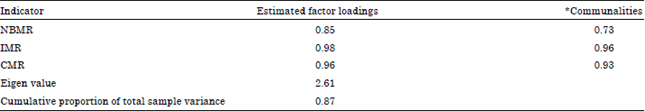
Table 1 shows the descriptive statistics for all three indicators of MF. The Pearson correlation values between NBMR and IMR, between NBMR and CMR, between IMR and CMR were found 0.73, 0.68 and 0.99, respectively. These correlations were found significant at p<0.001. The high significant of theses correlations indicates the high consistent in constructing the MF. Table 2 shows the results of factor analysis.
The descriptive statistics were calculated for the MF. The mean and standard deviation of MF were found 0 and 1, respectively. The skewness and kurtosis were found 0.16 and -0.24, respectively. The five-number summary of the MF consisted of minimum, maximum and quartiles written in increasing order: Min = -1.81, Q1 = -0.77, Q2 = 0.02, Q3 = 0.87 and Max = 2.31. From the five-number summary, the variations of the four quarters were found 1.04, 0.79, 0.85 and 1.44, respectively. The results of Kolmogorov-Smirnov normality test for the MF were found: Statistic = 0.10 and p = 0.200 which confirms the normal distribution. Table 3 shows the transformed three indicators (NBMR, IMR and CMR), MF, local Moran values of the MF and its p-values based on simulation study under standard normal distribution.
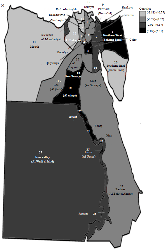
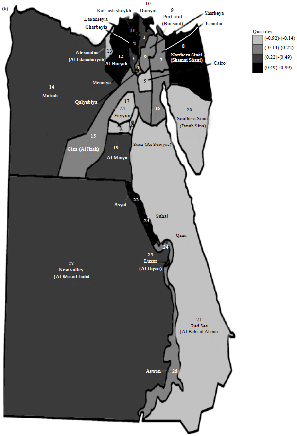
Figure 2a-b show visual insight for the MF and its local Moran values, respectively. Darkest shade corresponds to the highest quartile. These maps display geographical variation across Egypt’s governorates. Based on visual inspection for the MF taken from Figure 2a, an overall worsening pattern (higher scores) was found in the eastern-northern, middle and southern governorates. The hypothesis of global spatial clustering of the MF that follows a visual inspection of mapping was not confirmed by a positive significant global Moran’s I of 0.15 with an associated z-statistic of 1.76, p = 0.79 and permutation p = 0.068.
| Table 1: | Descriptive statistics, round it to two digits, for all indicators before and after transformation into the normal distribution |
 | |
| Table 2: | Results of factor analysis |
 | |
| *Communality is the proportion of a variable’s variance explained by the retained factors | |
  | |
| Fig. 2(a-b): | Choropleth maps show (a) MF and (b) Its local Moran values |
| Table 3: | Three transformed indicators, MF, local moran values and its p-values, where the p-value in boldface was considered significant at 0.05 level |
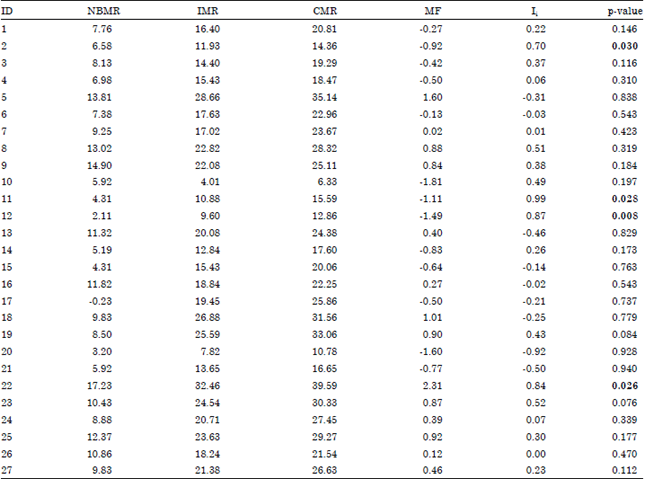 | |
Accordingly, the null hypothesis of no spatial autocorrelation was not rejected. Although, this finding was not expected, four significant local clusters were found (they are: Gharbeyia, Kafr ash Shaykh, El Buhayrah and Asyut) as shown from their p-values in boldface in Table 3.
DISCUSSION
The author investigated the spatial pattern of children mortality in Egypt in 2007. The spatial global clustering and local clusters for the MF were examined based on global Moran’s I and local Moran’s Ii, respectively. The large inequality in the risk of child mortality is a major challenge facing the government of Egypt. To reduce this inequality, accessibility to health services needs to be improved to poorer members of the population. The decentralization of many former central government responsibilities provides an opportunity to make such improvements.
The above framework revealed some noteworthy findings. Such findings allow policy makers to better identify what types of resources are needed and precisely where they should be employed. After do not reject the null hypothesis, concluding that there is no form of global clustering in the MF, it is of course, of interest to know the exact nature of this clustering. Are there hot-spot clusters? If so, how many hot-spots are there and where they are located? The population size in the governorates is not equal i.e., the three indicators NBMR, IMR and CMR were not expressed the absolute size of the inequality problem. Several governorates were not observed visually as hot spots. But after considering the information of their neighbours, the pattern of their hot spots can be obviously seen; for example, governorates 2, 11 and 12.
Anselin (1995) stated that the indication of local pattern of spatial association may be in line with a global indication, although this is not necessarily be the case. It is quite possible that the local pattern is an aberration that the global indicator would not pick up, or it may be that a few local patterns run in the opposite direction of the global spatial trend. Local values that are very different from the mean (or median) would indicate locations that contribute more than their expected share to the global statistic. These may be outliers or high leverage points and thus would invite closer scouting. However, this case was found in this research. Although, the global clustering in the MF was not found significant, four local clusters were found significant. One potential explanation for this variation in child mortality risk is the differences in socio-economic status in the population. Access to maternal and child health services that can reduce the risk of child mortality can probably explain this variation. Surjadi (2002) found that the proximity of residents to health facilities influences their usage of them. In Egypt due to expensive private health facilities are perceived to be of higher quality than public health services, they can therefore be assumed to be better at reducing child mortality risk.
The spatial analysis units are arbitrary subdivisions of the study region and the people could move around from one area to another. So, the people could be affected by the mortality in the governorate other than the governorate they live in i.e., the mortality the ith governorate is thought to be influenced and explained by the mortality not just in the ith governorate but also in its neighbouring governorates.
The map provides powerful means to communicate the data to others. Unlike information displayed in the graphs, tables and charts: The map also provides bookmarks for memories. In this way, the map is not a passive mechanism for presenting the information. Usually, in the spatial analysis and geographical mapping, small areas are used such as districts, counties…etc. But in this research governorates were used which considered somewhat larger than for example the districts because the data were not available for smaller areas. The results from population datasets are very sensitive to how the spatial units are constructed. Usually, if different spatial units are used different results will obtain. The larger the spatial units are used, the larger inequality is obscured. Most often the word ‘neighbourhood’ suggests a relatively of small area surrounding individuals’ homes. But researchers commonly make use of larger spatial area such as census tracts (Coulton et al., 2001). Often, the choice about neighbourhood spatial definition was made with respect to the convenience and availability of contextual data rather than study purpose as stated by Schaefer-McDaniel et al. (2010). They noted researchers might utilize census data and thus rely on census-imposed boundaries to define neighbourhoods even though these spatial areas may not be the best geographic units for the study topic. Also, many studies in geography have demonstrated that results can vary according to scale and configuration of spatial units.
As noted by Waller and Jacquez (1995), the test for spatial pattern employs alternative hypotheses of two types; the omnibus not the null hypothesis or more specific alternatives. Tests with specific alternatives include focused tests that are sensitive to monotonically decreasing risk as distance from a putative exposure source (the focus) increases. Acceptance of either types (the omnibus or a more specific alternatives) only demonstrates that some spatial pattern exist and does not implicate a cause (Jacquez, 2004). Hence, the existence of a spatial pattern alone cannot demonstrate nor prove a causal mechanism.
The application of statistical techniques to spatial data faces an important challenge, as expressed in the first law of geography as stated by Tobler (1979): “Everything is related to everything else but closer things are more related than distant things”. The quantitative expression of this principal is the effect of spatial dependence i.e., when the observed values are spatially clustered, the samples are not independent. The MF growth in governorate i generates MF growth in governorate j. This mechanism of transmission causes a spatial autocorrelation in the MF growth. The obvious question after finding significant clusters in the MF is-why? Could this pattern is associated with the spatial pattern of other socioeconomic indicators such as the level of household income or with the limitation of economic resources? However, further research regarding this bivariate spatial association between the MF and other socioeconomic factors is required. This study adds to the global body of knowledge on the utilization of spatial analysis to strengthen the research-policy interface in the developing countries such as Egypt.
It should be emphasized that the problem of mortality inequality cannot be overcome in the short-run but long-term efforts are needed to tackle this problem. In turn, enabling the economy to create more job opportunities and establish new projects, especially in the governorates that found as hot spot clusters in mortality. It means that the place of the problem is now clearly shown. The lack of investment in all levels of education and other life skills results in permanent life-long inequality problem. That’s why, mortality studies should be conducted periodically in light of the changing of socioeconomic and political conditions. Chandola (2012) concluded the increasing spatial isolation of the poor people and areas tend to be associated with higher mortality rates using multiple Poisson regression models.
Details in this research enables development actors to identify priorities, select fields and locate trends in designing national, regional or sectorial policies. Moreover, this study provides civil society organizations, researchers and citizens with a rich knowledge base of facts and analysis, offering information easy to understand and to apply. This knowledge can be used either in targeted initiatives or as a tool for monitoring and assessing policies and methods. Most importantly, this research provides the information needed to both examine development strategies’ consistency with the actual situation and to align priorities and develop them in accordance with the Egyptian people’s development needs.
The significance of this study is showing how many spatial clusters in children mortality are existed and where they are located. This can greatly aid unpacking the understanding of neighbourhood relationship between health and environment. Although, this study was conducted as part of a larger research program, its immediate implications are more for policy makers and practitioners than for researchers. Policy which pays attention to the area characteristics will reduce the mortality inequality. Consequently, this will improve the health status. To reduce the risk of mortality in Egypt and other countries, efforts should focus on hot spot governorates rather than on all governorates.
CONCLUSION
Conclusion is comprehensive in at least four aspects. First, based on the visual inspection of mapping, the high level of children mortality was concentrated in eastern-northern, middle and southern governorates. Second, several governorates were not observed visually as hot spots. But after considering the information of their neighbours, the pattern of their hot spots can be obviously seen. Third, the global clustering was not found in children mortality, but four governorates were found to be local clusters in the northern and southern governorates. The opposite was for those governorates that have low mortality were seen in some middle and eastern-southern governorates. Forth, from negative local Moran values, looking at the local variation, some governorates represented as governorates of dissimilarity. These governorates were found to have low mortality were surrounded by governorates that have high mortality, or vice versa. In summary, the present study has supported the hypothesis of a spatial inequality in children mortality at governorate level in Egypt. Probably, this reflects the inequality distribution in several socioeconomic indicators across governorates of Egypt. While results were specific to the studied data, the case study helps to identify general concepts for future studies.
The results were consistent with the findings of previous studies taking into account the difference in the environment and the degree of growth of the Egyptian community. The characterization of neighbourhoods provides an overall guideline which can aid in issues such as health policy planning and development. Further studies are required to investigate the spatial relationship between children mortality and socioeconomic indicators. This study may be regarded as a first step in prioritizing areas for follow-up public health efforts.
REFERENCES
- Allender, S., P. Scarborough, T. Keegan and M. Rayner, 2012. Relative deprivation between neighbouring wards is predictive of coronary heart disease mortality after adjustment for absolute deprivation of wards. J. Epidemiol. Community Health, 66: 803-808.
CrossRef - Anselin, L., 1995. Local indicators of spatial association-LISA. Geograph. Anal., 27: 93-115.
CrossRefDirect Link - Auger, N., D. Hamel, J. Martinez and N.A. Ross, 2012. Mitigating effect of immigration on the relation between income inequality and mortality: A prospective study of 2 million Canadians. J. Epidemiol. Community Health, Vol. 66.
CrossRef - Bellec, S., D. Hemon, J. Rudant, A. Goubin and J. Clavel, 2006. Spatial and space-time clustering of childhood acute leukaemia in France from 1990 to 2000: A nationwide study. Br. J. Cancer, 94: 763-770.
CrossRef - Chandola, T., 2012. Spatial segregation and socioeconomic inequalities in health in Brazilian cities: Combining spatial and social epidemiology. J. Epidemiol. Community Health, 66: A1-A2.
CrossRef - Coulton, C.J., J. Korbin, T. Chan and M. Su, 2001. Mapping residents perceptions of neighborhood boundaries: A methodological note. Am. J. Community Psychol., 29: 371-383.
CrossRefDirect Link - Gupta, M.D., 1990. Death clustering, mother's education and the determinants of child mortality in rural Punjab, India. Popul. Stud. J. Demogr., 44: 489-505.
CrossRefDirect Link - Jacquez, G.M., 2004. Current practices in the spatial analysis of cancer: Flies in the ointment. Int. J. Health Geograph., Vol. 3.
Direct Link - De Pedro-Cuesta, J., E. Rodriguez-Farre and G. Lopez-Abente, 2009. Spatial distribution of Parkinson's disease mortality in Spain, 1989-1998, as a guide for focused aetiological research or health-care intervention. BMC Public Health, Vol. 9.
CrossRef - Johnson, R.A. and D.W. Wichern, 2002. Applied Multivariate Statistical Analysis. 5th Edn., Prentice Hall, Hoboken, New Jersey, ISBN: 9780130925534, Pages: 767.
Direct Link - Luginaah, I., M. Jerrett, S. Elliott, J. Eyles and K. Parizeau et al., 2001. Health profiles of Hamilton: Spatial characterisation of neighbourhoods for health investigations. GeoJournal, 53: 135-147.
CrossRef - Macintyre, S., S. Maciver and A. Sooman, 1993. Area, class and health: Should we be focusing on places or people? J. Social Policy, 22: 213-234.
CrossRef - Sankoh, O.A., Y. Ye, R. Sauerborn, O. Muller and H. Becher, 2001. Clustering of childhood mortality in rural Burkina Faso. Int. J. Epidemiol., 30: 485-492.
CrossRefDirect Link - Schaefer-McDaniel, N., M.O. Caughy, P. O'Campo and W. Gearey, 2010. Examining methodological details of neighbourhood observations and the relationship to health: A literature review. Social Sci. Med., 70: 277-292.
CrossRefPubMedDirect Link - Waller, L.A. and G.M. Jacquez, 1995. Disease models implicit in statistical tests of disease clustering. Epidemiology, 6: 584-590.
Direct Link