
Kufre J. Bassey
Department of Mathematical Sciences, Federal University of Technology, P.M.B. 704, Akure, Ondo State, Nigeria
Trends in Applied Sciences Research
Year: 2011 | Volume: 6 | Issue: 11 | Page No.: 1293-1300


ABSTRACT
Compared with other sources of pollution in the oceans, the risk of crude oil spillage to the sea presents the major threat for the marine ecology. There is no doubt the fact that there are sophisticated instruments like photoacoustic instrumentation for measuring oil in water bodies. Since oil start spreading immediately it enters water, it follows that spilled oil in water bodies is a state with incomplete information which therefore requires state estimation. This study uses Bayesian Statistics in deriving a linear unbiased minimum-error-variance algorithm for estimating the state of oil in water bodies. This is essential especially when chemical dispersant is a control alternative, given that this substance may have its own effect on marine biomass.
PDF Abstract XML References Citation
Received: February 25, 2011;
Accepted: June 22, 2011;
Published: September 06, 2011
How to cite this article
Kufre J. Bassey, 2011. A Linear Unbiased Minimum-Error-Variance Algorithm for Marine Oil Spill Estimation. Trends in Applied Sciences Research, 6: 1293-1300.
URL: https://scialert.net/abstract/?doi=tasr.2011.1293.1300
URL: https://scialert.net/abstract/?doi=tasr.2011.1293.1300
INTRODUCTION
Petroleum products that enter the marine environment have distinct effects, according to their composition, concentration and the element that are considered (Steinberg et al., 1997). The severity of these effects varies from disastrous to no detectable impacts. Akpovire (1989) and Yapa et al. (1994) highlighted possible causes of oil spills to include oil transport; oil exploration; inland navigation and oil storage facilities. Review of global oil spills incidence shows that marine oil spills also play a significant role in the world economic and environmental devastation (Cekirge et al., 1992).
As a case in point when oil is spilled on water, the transport and fate of the spilled oil are governed by the physical, chemical and biological processes that depend on the oil properties, hydrodynamics, meteorological and environmental conditions (ASCE Task Committee on Modeling of Oil Spills of the Water Resources Engineering Division, 1996). The processes include advection, turbulent diffusion; surface spreading; evaporation; dissolution; emulsification; hydrolysis; photo-oxidation; biodegradation and particulation (Tkalich, 2002).
On the sea surface, the oil spreads to form a thin film called oil slick. The movement of the slick is governed by the advection and turbulent diffusion due to current and wind actions (Maged and Ibrahim, 1999). The slick spreads over the water surface due to a balance between gravitational, inertial, viscous and interfacial tension forces and the composition of the oil changes from the initial time of the spill (Tkalich and Chao, 2001).
The physical and chemical changes which spilled oil undergo are sometimes collectively known as weathering. During this process, light fractions of the oil evaporate water soluble components dissolve in the water column and the immiscible components become emulsified and dispersed in the water as droplets. Thus, the severity of environmental impacts resulting from this weathering process varies from disastrous to no detectable effect, depending upon the quantity of hydrocarbons released, the physio-chemical properties of oil, the nature of the incident and its proximity to the shoreline (Lyman et al., 1990; Clark, 1996).
This threat of economic and environmental devastation by petroleum products that enters marine environments has lead to the development of a number of clean-up alternatives which may be grouped as: (i) recovery of oil from the sea surface with mechanical devices (ii) dispersion of oil into the water column with chemical dispersants and (iii) sinking of oil with heavier-than-water materials. Among these three categories, only category one does not require the addition of chemical to the water, yet it is not always effective, especially for longer range planning (Dewling and McCarthy, 1981; Etkin, 1999). A significant problem in solving environmental issues is related to the issues of integrated environmental management (Magram, 2009). Thus, the aim of this study is to develop a linear unbiased minimum-error-variance algorithm for estimating the state of oil in water bodies which will serve as a guide for optimal decision strategy with respect to oil spill clean-up alternatives.
CHEMICAL DISPERSANT AS CONTROL TOOL
On like other water disinfection methods (Ibeto et al., 2010), chemical dispersants are mixtures of solvents, surfactants and other additives that are applied to oil slicks to reduce the oil-water interfacial tension (Clayton et al., 1993). The reduction of interfacial tension between oil and water by addition of a chemical dispersant promotes the formation of a larger number of small oil droplets when surface waves entrain oil into the water column. These small submerged oil droplets are then subjects to transport by subsurface currents and other weathering process such as evaporation, dissolution, biodegradation, etc. It is evident in the literature that the presence of dispersant enhanced crude oil biodegradation (Zahed et al., 2010). The use of dispersant in oil spill cleanup has also shown a significant reduction in the overall cleanup cost (Etkin, 1998). Nevertheless, recent studies suggest that toxicity from physically and chemically dispersed oil appears to be primarily associated with the additive effects of various dissolved-phase Polynuclear Aromatic Hydrocarbons (PAH) with additional contributions from heterocyclic (N, S and O) containing polycyclic aromatic compounds. Additional toxicity may be coming from the particulate or oil droplet, phase but a particular concern stems from potential synergistic effects of exposure to dissolved components in combination with chemically dispersed oil droplets (Humphrey, 2010).
STATISTICAL ESTIMATION TECHNIQUE
In statistics, estimation theory is a basic tool used in system and control theory. When spill occurs in soil or sea, it constitutes part of the events happening in that system. These events generate messages which require observations at a receiver (Cheng et al., 2008). The messages and the observations are stochastically related. The objective in the event of spill is to determine a strategy or a rule which forms a best guess of the message based on the observation. Let M be the message space which is a subset of a Euclidean space. The message of oil spill therefore involves selecting a message, such as the amount of oil m in the observed location from M. The problem is to determine the value of m from the observation in some optimal fashion. It is known that the moment oil is spilled into water bodies, it starts spreading immediately. Thus, a good estimation of the amount of oil in the system requires some certain level of observation, y which can only be done through a noisy channel. In this case, statistical estimation technique is required in trying to determine the value of m.
Definition: Estimation is an aspect of inference whereby some information (statistic) are obtained from a sample which helps in determining (estimating) the corresponding parameter of the population from which the sample was drawn. A function of the elements of the sample used in making a good guess of the unknown parameter is called an estimator. Thus, the numerical value of the estimator obtained from the sample data is referred to as an estimate.
Estimation is a necessary condition for optimal prediction (Tzimopoulos et al., 2008). The focus of this study is to estimate a time-varying state of spilled oil in water bodies using a linear unbiased minimum-error-variance sequential-state estimation algorithm known as Kalman filter and the performance index of the system after a control has been applied using maximum likelihood estimation technique.
The algorithm: Consider the development of a linear unbiased minimum-error-variance recursive algorithm for estimating the state xk of a state-space model at time k given the values of the observed outputs yk-1 = (y0, y1,…, yk-1). This state is called ‘the state of oil in water bodies’ which is described by the following linear vector model:
| (1) |
| (2) |
where, A (k), C (k), H (k) and G (k) are unknown and thus assumed time-varying coefficient matrices governed by a Gauss-Markov process, ek is an input or message white noise process with zero-mean and unit covariance (E [ek e'k] = I), lk is a zero-mean measurement white-noise process with unit covariance (E [lk l'k] = I). The initial state x0 is uncorrelated with the white noises and has a known mean μ0 and covariance V0 with the following assumption:
| (3) |
Equation 1 is called the message model given that it describes the basic information that is to be determined. Thus the state in question xk is observed by means of noisy mechanism defined as measurement model and given by Eq. 2. Let us denote by Vm, Vx and Vx, the covariance of the message white-noise process, the measurement white-noise process and the variance of the initial state x0, respectively. And also with the assumption that e and l are uncorrelated so that:
| (4) |
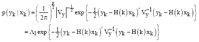
Hence, sequential observations should be conducted in the system up to the decision time k since the oil starts spreading immediately it is released. In what follows, a set of sequential observations Yk = (y1, y2,..., Yk) will be expected. The aim is to estimate x at k. So, to obtain a linear minimum-variance estimator, a Gaussian amplitude distribution for x, e and l which makes the Kalman filter the best (minimum-error-variance) linear filter is assumed (Kalman and Bucy, 1961; Van Trees, 1968; Anderson and Moore, 1979). To derive the Kalman filter algorithm for this kind of estimation, it is noted that getting measurement for the state of oil in water x at time k is conditioned on the observations up to time k (i.e., Yk) which is a chance event. Therefore, Bayes’ technique is employed and the maximum a posteriori procedure which gives the estimate of xk|yk as the value of x at time k which maximizes the probability p (xk|yk) in every realization of x is utilized. This is done by first expressing:
| (5) |
Then by setting Yk to denotes all observation up to time (k-1) and that of time k, Eq. 5 becomes:
| (6) |
One can write:
| (7) |
| (8) |
which follows from the joint probability law. Putting Eq. 8 in Eq. 6 gives:
| (9) |
Equation 9 can be written following the probability law as:
| (10) |
But the objective is to determine xk given Yk. Thus, the probability p (yk|xk) needs to be examined. To do this, the expectation of (yk|xk) is first considered:
| (11) |
then its variance:
| (12) |
So that:
 | (13) |
Next, the expectation of the density p (xk|yk-1) is considered as follows:
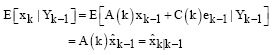 | (14) |
where, ![]() is the unbiased estimator of x at time y and the variance:
is the unbiased estimator of x at time y and the variance:
| (15) |
Again, one can write:
| (16) |
So that:
| (17) |
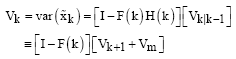
where, Vk-1 = var ![]()
Thus:
| (18) |
where,
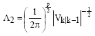 |
Putting Eq. 13 and 18 in Eq. 10 it becomes:
| (19) |
And then, applying the maximum a posteriori procedure it gives:
| (20) |
| (21) |
Thus:
| (22) |
It then follows from matrix inversion lemma (Hannan et al., 1980; Sage and Melsa, 1971; Hastings-James and Sage, 1969) that:
| (23) |
where,
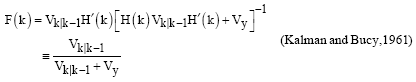 | (24) |
and is called the Kalman gain. The filtering error is given by:
| (25) |
If Eq. 22 is substituted into Eq. 25 and Eq. 2 recalled, the following is obtained:
| (26) |
and the error variance given by:
 | (27) |
Finally, the Kalman filter algorithm derived above can be summarized as:
| • | Initialization: |
| • | Backward: Message model: xk = A (k) xk-1+ek |
| • | Given a sequence of observation yk-1 = (y0, y1,…, yk-1), for k>0, compute Eq. 14 |
| • | Forward: Message model: xk-1 = xk+ek |
To implement the Kalman filter, compute the sequence Vk from Eq. 27 and the corresponding sequence F (k) using Eq. 24. Computation of ![]() can then be done recursively using Eq. 14 as successive observations become available.
can then be done recursively using Eq. 14 as successive observations become available.
CONCLUSION
In disaster emergency management of chemical pollutant like oil spill, spill volume or amount is the most difficult to determine or estimate (El-Shenawy et al., 2010). For example, in the case of a vessel accident, the exact volume in a given compartment may be known before the accident but the remaining oil may have been transferred to other ships immediately after the accident. Sometimes the exact character or physical properties of the oil lost are not known and this leads to different estimations of the amount lost. For optimal response to oil spill cleanup in marine environment, there is need to have a good estimate of the state variable for a better strategic decision-making. When the state of a system is unknown or partially known, there are two main situations that are responsible: first, restrictions on the system observability and secondly, restrictions on the system controllability. Consequently when the system variables are subject to theoretical observability and controllability restrictions, an estimation problem results. The control problem can be solved by reconstructing the system state variables. This can be carried out by using the Kalman filter. Least squares estimators are therefore recommended because they are minimum variance linear unbiased estimators which also permit easy computation and readily modify to yield recursive estimators of the Kalman filter form when new information is available. This can be achieved through the following procedure:
| • | Determine the parameter of the system at each time period by least-squares method based on all available data |
| • | Determine the control policy for the model estimated at step 1 |
| • | Repeat step 1 and 2 at each succeeding sampling interval |
The updating of the parameter estimates allows the accuracy of the control to be improved at each step.
REFERENCES
- ASCE Task Committee on Modeling of Oil Spills of the Water Resources Engineering Division, 1996. State-of-the-art review of modeling transport and fate of oil spills. J. Hydraul. Eng., 122: 594-609.
CrossRefDirect Link - Cheng, D., L. Zhaoxia, Y. Jinlong and J. Jianxiang, 2008. Adsorption behavior of p-chlorophenol on the reed wetland soils. J. Environ. Sci. Technol., 1: 169-174.
CrossRefDirect Link - El-Shenawy, N.S., Z.I. Nabil, I.M. Abdel-Nabi and R. Greenwood, 2010. Comparing the passive and active sampling devices with biomonitoring of pollutants in langstone and portsmouth harbour, UK. J. Environ. Sci. Technol., 3: 1-17.
CrossRefDirect Link - Etkin, D.S., 1999. Estimating cleanup costs for oil spills. Proceedings of the 1999 International Oil Spill Conference, March 8-11, Seattle, Washington, USA., pp: 35-39.
Direct Link - Ibeto, C.N., N.F. Oparaku and C.G. Okpara, 2010. Comparative study of renewable energy based water disinfection methods for developing countries. J. Environ. Sci. Technol., 3: 226-231.
CrossRefDirect Link - Kalman, R.E. and R.S. Bucy, 1961. New results in linear filtering and prediction theory. ASME Trans. D: J. Basic Eng., 83: 95-108.
Direct Link - Hannan, E.J., W. Dunsmuir and M. Deistler, 1980. Estimation of vector ARMAX models. J. Multivariate Anal., 10: 275-295.
CrossRef - Magram, S.F., 2009. A review on the environmental issues in Jeddah, Saudi Arabia with special focus on water pollution. J. Environ. Sci. Technol., 2: 120-132.
CrossRefDirect Link - Steinberg, L.J., K.H. Reckhow and R.L. Wolpert, 1997. Characterization of parameters in mechanistic models: A case study of a PCB fate and transport model. Ecol. Modell., 97: 35-46.
CrossRef - Tzimopoulos, C., L. Mpallas and G. Papaevangelou, 2008. Estimation of evapotranspiration using fuzzy systems and comparison with the blaney-criddle method. J. Environ. Sci. Technol., 1: 181-186.
CrossRefDirect Link - Yapa, P.D., H.T. Shen and K.H. Angammana, 1994. Modeling oil spills in a river-lake system. J. Mar. Sci., 4: 453-471.
CrossRef - Zahed, M.A., H.A. Aziz, H.M. Isa and L. Mohajeri, 2010. Effect of initial oil concentration and dispersant on crude oil biodegradation in contaminated seawater. Bull. Environ. Contam. Toxicol., 84: 438-442.
CrossRefDirect Link