INTRODUCTION
Cocoa, scientifically known as Theobroma cacao L. is the third-largest
agricultural commodity in Malaysia after oil palms and rubber. Malaysia now
exports cocoa products to sixty-six countries (Ministry of
Plantation Industries and Commodities, 2006). Tawau is one of the top cocoa
producers in Malaysia and even in the world along with the Ivory Coast, Ghana
and Indonesia (Shanti, 2006). Domestic cocoa bean prices
are changing from time to time and very volatile (Yusoff
and Salleh, 1987; Arshad and Zainalabidin, 1994).
Instability of cocoa prices creates significant risks to producers, suppliers,
consumers and other parties that are involved in the marketing and production
of cocoa beans, particularly in Malaysia. In risky conditions and amidst price
instability, forecasting is very important in helping to make decisions. Accurate
price forecasts are particularly important to facilitate efficient decision
making as there is time lag intervenes between making decisions and the actual
output of the commodity in the market.
Modelling or forecasting of agricultural price series, like that of other economic
time series, has traditionally been carried out either by building an econometric
model or by applying techniques developed for analyzing stationary time series.
Time series forecasting is a major challenge in many real world applications
such as stock price analysis, palm oil prices, natural rubber prices, electricity
prices and flood forecasting. This type of forecasting is to predict the values
of a continuous variable (called as response variable or output variable) with
a forecasting model based on historical data. There are two types of time series
forecasting modeling methods; univariate and multivariate. Univariate modeling
methods generally used time only as an input variable with no other outside
explanatory variables (Celia et al., 2003). This
forecasting method is often called univariate time series modeling. A few commonly
employed methods in univariate time series models are exponential smoothing,
autoregressive-integrated-moving average (ARIMA) and Autoregressive Conditional
Heteroscedastic (ARCH) (Kahforoushan et al., 2010).
The last few decades have witnessed significant advances in the topic of exponential
smoothing. It has established itself as one of the leading forecasting strategies
(Robert and Amir, 2009). Fatimah
and Roslan (1986) confirmed the suitability of univariate ARIMA models in
agricultural prices forecasting. Shamsudin et al.
(1992) has noted that ARIMA models have the advantage of relatively low
research costs when compared with econometric models, as well as efficiency
in short term forecasting. One of the earliest time series models allowing for
heteroscedasticity is the Autoregressive Conditional Heteroscedastic (ARCH)
model introduced by Engel (1982). Bollerslev
(1986) extended this idea into Generalized Autoregressive Conditional Heteroscedastic
(GARCH) models which give more parsimonious results than ARCH models, similar
to the situation where ARMA models are preferred over AR models. Kamil
and Noor (2006) have developed a time series model of Malaysian palm oil
prices by using ARCH models. Zhou et al. (2006)
have proposed a new network traffic prediction model based on non-linear time
series ARIMA/GARCH. They found that the proposed ARIMA/GARCH outperformed the
existing Fractional Autoregressive Integrated Moving Average (FARIMA) model
in terms of prediction accuracy. Therefore, the objective of this research was
to compare the forecasting performances of four different univariate time series
methods or models for forecasting cocoa bean prices (i.e., Tawau cocoa bean
prices), namely exponential smoothing, ARIMA, GARCH and the mixed ARIMA/GARCH
models.
MATERIALS AND METHODS
The monthly Tawau cocoa bean prices graded SMC 1B was used for this study which
was collected from the official website of The Malaysian Cocoa Board (http://www.koko.gov.my/lkmbm/loader.cfm?page=statisticsFrm.cfm).
The time series data was measured in Ringgit Malaysia per tonne (RM/tonne).
The time series data ranged from January 1992 until December 2006. The coefficient
of variation (V) was used to measure the index of instability of the time series
data. The coefficient of variation (V) is defined as:
where σ is the standard deviation and
is the mean of Tawau cocoa bean prices changes.
A completely stable data has V = 1, but unstable data are characterized by
a V>1 (Telesca et al., 2008).
Regression analysis was used to test whether trends and seasonal factors exist in the time series data. The existence of linear trend factors was tested through this regression equation
with Y is the time series data of the study, Trend is the linear trend factor, β0 and β1 are parameters and ε is the error of the model with an assumption of White Noise (WN). The hypothesis of the model was
• |
H0: β1 = (Non-existence
of linear trend factor) |
• |
H1: β1≠ (Linear trend factor
exists) |
With the month of January as the base month, the existence of seasonal factor
was detected by using regression as shown below:
and hypothesis was defined as:
• |
H0: β2 = β3
= β4 = ...β12 = 0 (Non-existence of seasonal
factor) |
• |
H1: At least one of β2,
β3, ..., β12≠ 0 (Seasonal factor exists) |
The correlogram and Augmented Dickey-Fuller (ADF) test were chosen to test
the stationary of the time series data.
Exponential Smoothing
The h-periods-ahead forecast is given by:
with a and b are permanent components. Both of these parameters are counted by the following equations
with 0<α, β<1.
ARIMA
This study followed the Box-Jenkins methodology which involves four steps. These are identification, estimation, model checking and forecasting. ARMA (p, q) processes can be simply expressed as the following two Eq.
where, xt is the explanatory variables, etis the disturbance term, εt is the innovation in the disturbance, p is the order of AR term, q: the order of MA term. In Eq. 2, the disturbance term (μt) again consists of three parts. The first part is AR terms and the second part is MA terms. The last one is just a white-noise innovation term. If we replace the data (Y) with the difference data (Δyt = Yt-Yt-1), then the ARMA models become ARIMA(p, d, q) models.
GARCH
The standard form of GARCH(p,q) models can be specified as following three equations:
where, p is the order of GARCH term, q is the order of ARCH term and σ2v.
Equation 3 and 5 are called mean equation
and conditional variance equation, respectively. The mean equation is written
as a function of exogenous variables (xt) with an error term (μt).
The variance equation is a function of mean (δ), ARCH (μ2t-i)
and GARCH term (μ2t-t).
ARIMA/GARCH
Combination of ARIMA(p,d,q) and GARCH(p,q) are written as below:
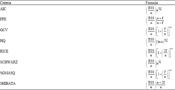
Eight model selection criteria as suggested by Ramanathan
(2002) were used to chose the best forecasting models among ARIMA and GARCH
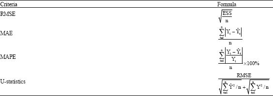
models (Table 1). While, the best time series methods for
forecasting Tawau cocoa bean prices was chosen based on the values of four criteria,
namely RMSE, MAE, MAPE and U-statistics (Table 2). Finally,
the selected model was used to perform short-term forecasting for the next twelve
months for Tawau cocoa bean prices starting from January 2007 until December
2007.
Table 1: |
Model Selection Criteria (Ramanathan, 2002) |
 |
n: Number of observations, f: Number of parameters, ESS: Error
sum of square |
Table 2: |
Forecast accuracy criteria |
 |
Yt: The actual value at time t, :
The forecast value at time t, n: The number of observations; ESS: The error
sum of square |
RESULTS
The results showed that the coefficient of variation (V) of the time series
data was 1.012 (V>1). Because of the V value was closed to 1, so this study
was concluded that the time series data was stable (Telesca
et al., 2008). The results of the regression analysis have shown
that positive linear trend factor exists in the time series data but seasonal
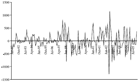
factor was not. With referring to the correlogram and the Augmented Dickey-Fuller
tests results, the time series data of the study was not stationary. But after
the first order of differencing was carried out, the time series data became
stationary (Fig. 1).
Exponential Smoothing
The double exponential smoothing method was used as the regression result
has showed the positive linear trend factor exists in the time series data.
Double exponential smoothing models consist with two parameters which symbolized
as α for mean and β for trend. The best model of the double exponential
smoothing has been selected based on the lowest value of MSE (Mean Square Error)
from combination of α and β with condition 0<α, β<1.
|
Fig. 1: |
Time series data (after first order of differencing) |
Table 3: |
Error Sum of Square (ESS) according to α and β
values |
 |
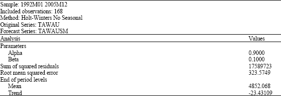
Table 4: |
EViews output of the double exponential smoothing model |
 |
The result showed that combination α = 0.9 and β = 0.1 was the best
forecasting model of double exponential smoothing method (Table
3). The double exponential smoothing model was written in equation form
as (Table 4).
ARIMA
All models which fulfilled the criteria of p+q≤5 have been considered and
compared in this study and there were twenty ARIMA (p, d, q) models which fulfilled
the criteria. Parameters of the models were estimated with the least square
method. Parameters which were not significant at 5% confidence level were dropped
from the model. Using the eight model selection criteria suggested by Ramanathan
(2002), the ARIMA (3, 1, 2) model was selected as the best model among the
other ARIMA models. However, the parameters of AR (1) and MA (1) were found
not significant and thus dropped from the model.
Table 5: |
Estimation of ARIMA (3, 1, 2) |
 |
*p<0.05 |
Table 6: |
Estimation of GARCH (1, 1) |
 |
*p<0.05 |
Table 7: |
Estimation of ARIMA (3, 1, 2)/GARCH (1, 1) |
 |
*p<0.05 |
The ARIMA (3, 1, 2) model was written in equation form as (Table
5).
GARCH
Identification and estimation of GARCH (p, q) models in this study were done
by following the four steps that were ARCH effect checking, estimation, model
checking and forecasting. Four GARCH (p,q) models were selected and compared,
namely GARCH (1, 1), GARCH (1, 2), GARCH (2, 1) and GARCH (2, 2). Using the
eight model selection criteria suggested by Ramanathan (2002),
the GARCH (1, 1) model has been selected as the best model among the other three
GARCH models.
The GARCH(1,1) model was written in equation form as (Table 6):
ARIMA/GARCH
ARCH effect which was tested by using a regression analysis exists in the ARIMA (3, 1, 2) model. That means the ARIMA (3, 1, 2) model could be mixed with the best GARCH model (i.e., GARCH(1, 1)).
The ARIMA(3, 1, 2)/GARCH(1, 1) model was written in equation form as (Table 7):
Table 8: |
Four model selection criteria |
 |
|
Fig. 2: |
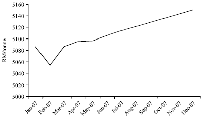
Short-term forecasting of tawau cocoa bean prices |
Model Selection
Four model selection criteria were used to select the best forecasting model
from the four different types of time series methods. Based on the results of
the ex-post forecasting (starting from January until December 2006), the ARIMA
(3, 1, 2)/GARCH (1, 1) model was the best short-term forecasting model of Tawau
cocoa bean price graded SMC 1B (Table 8).
Ex-Ante Forecasting
Based on the ex-ante forecasting by using the mixed ARIMA/GARCH model, Fig.
2 shows that the short-term forecasting indicated an upward trend of Tawau
cocoa bean prices for the period January-December 2007.
DISCUSSION
The result showed that the time series data (starting January 1992 until December
2006) was stable. This is contradict with the previous researches (Yusoff
and Salleh, 1987; Arshad and Zainalabidin, 1994)
which stated that domestic cocoa bean prices are changing from time to time
and very volatile. The results of the regression analysis have shown that positive
linear trend factor exists in the time series data but seasonal factor was not.
That means the cocoa bean prices of Tawau have increased in the period of 1992-2006
but seasonal factor which is usually related to climate change has not given
any significant influence on the monthly changes of cocoa bean prices. The mixed
ARIMA/GARCH model outperformed the exponential smoothing, ARIMA and GARCH for
the case of forecasting monthly Tawau cocoa bean prices. This is in agreement
with the findings in the literature (Zhou et al., 2006).
Some of previous research have found that ARIMA models (Fatimah
and Roslan, 1986; Shamsudin et al., 1992;
Kahforoushan et al., 2010) and also GARCH-type
models (Kamil and Noor, 2006) were the best or suitable
price forecasting models in terms of prediction accuracy, but the accuracy of
the mixed ARIMA/GARCH should also be considered in price forecasting for the
future researches.
CONCLUSION
This study investigates four different types of univariate time series methods, namely exponential smoothing, ARIMA, GARCH and the mixed ARIMA/GARCH. The results showed that the mixed ARIMA/GARCH model outperformed the exponential smoothing, ARIMA and GARCH for forecasting Tawau cocoa bean prices. Forecasting the future prices of cocoa bean through the most accurate univariate time series model can help the Malaysian government as well as the buyers (e.g., exporters and millers) and sellers (e.g., farmers and dealers) in cocoa bean industry to perform better strategic planning and also to help them in maximizing revenue and minimizing the cost of price.