
M. Azadi
Atmospheric Science and Meteorological Research Center, P.O. Box 14977-16385, Tehran, Iran
Z. Zakeri
I.R. Iran Meteorological Organization, P.O. Box 13185-461, Tehran, Iran
Research Journal of Environmental Sciences
Year: 2010 | Volume: 4 | Issue: 2 | Page No.: 138-148


ABSTRACT
An attempt is made to produce probabilistic precipitation forecasts from deterministic model output over Iran. Due to the chaotic nature of the atmosphere, probabilistic weather forecasts can be used to quantify the intrinsic uncertainty in the output of meteorological forecasting models. Probabilistic forecasts are more flexible to use and of greater economic value to data users when compared to deterministic forecasts. In this study, the results of the application of a simple and practical method for converting deterministic precipitation forecasts into probabilistic forecasts are presented. The model prediction for precipitation in the spatio-temporal neighborhood around each grid point is used to calculate the probability of precipitation at that point. The method was applied to the Pennsylvania State University-NCAR Mesoscale Model version 5 (MM5) precipitation forecasts for January 2005 over Iran. The quality and economic value of probabilistic forecasts was evaluated for 6 and 12 h accumulated precipitation forecasts. Results showed that the derived probabilistic forecasts were superior to the corresponding deterministic forecasts in quality, economic value and consistency. Also, since the method is easy to implement with minimal computational requirements, it is thus an affordable and appropriate method for operational implementation in a variety of settings.
PDF Abstract XML References Citation
How to cite this article
M. Azadi and Z. Zakeri, 2010. Probabilistic Precipitation Forecasting using a Deterministic Model Output over Iran. Research Journal of Environmental Sciences, 4: 138-148.
DOI: 10.3923/rjes.2010.138.148
URL: https://scialert.net/abstract/?doi=rjes.2010.138.148
DOI: 10.3923/rjes.2010.138.148
URL: https://scialert.net/abstract/?doi=rjes.2010.138.148
INTRODUCTION
The results of Quantitative Precipitation Forecasts (QPFs) are most meaningful when expressed in a probabilistic framework in order to consider the uncertainty that originates from the chaotic nature of the atmosphere (Fritsch et al., 1998). Experienced forecasters intuitively use the entire output of deterministic models and its spatial distribution to forecast local phenomena, thereby incorporating uncertainty in a subjective way. One of the main characteristics of forecast quality is that the uncertainty, which is inherent in a forecaster’s judgment, is reflected in the forecast product (Murphy, 1993). A probabilistic forecast helps the user in a more appropriate way for a desirable decision making with more flexibility.
Ensemble forecasting is the most common approach for explicit treatment of uncertainty in weather forecasts (Du et al., 1997). Due to the fact that this method is complex and computationally expensive, simpler and more affordable methods have been employed for deriving probabilistic forecasts from deterministic outputs of models, including subjective interpretation by human forecasters (Hamill and Wilks, 1995; Krzysztofowicz and Sigrest, 1999), automated methods based on historical error statistics for the model (Applequist et al., 2002) and a combination of both approaches (Roulston and Smith, 2003; Bremnes, 2004).
In small operational forecasting centers, there are limitations on subjective interpretation and ensemble forecasting. Ensemble forecasting requires a large amount of computational power for multiple high resolution model runs. Subjective interpretation, on the other hand, requires qualified and experienced local forecasters. Approaches using statistical distributions of historical model error are not expensive, but establishing such methods requires a long history of consistent use of the same model and a substantial observational data archive covering a sufficient time span that are not always available. The method presented here is based on the approach proposed by Theis et al. (2005) for deriving probabilistic weather forecasts for grid points from direct model outputs.
The method described and applied here is aimed for calculating probabilistic precipitation forecasts from deterministic model output over Iran. The approach is based on the observation that information about precipitation at a given point in space and time can be derived from its spatio-temporal neighborhood. Postprocessing of model outputs is a useful tool for extracting additional information from these outputs with minimum added expense.
MATERIALS AND METHODS
Postprocessing Method
The approach for producing probabilistic forecasts proposed by Theis et al. (2005) and applied here over Iran for 9 to 11 January 2005 is briefly reviewed in the following. In order to derive a probabilistic postprocessed forecast (PPPF) for a given grid point (x0,y0) in the domain for time T0, a neighborhood in space and time around the grid point is first defined. Figure 1 shows a sample neighborhood in the (x,y) and (x,t) planes. Δx and Δy are grid distances in the x and y directions respectively and Δt denotes the selected time interval between successive model outputs.
The basic hypothesis underlying the postprocessing technique applied here is that the precipitation forecasts in the neighborhood of (x0,y0) are considered to be a sample of an unknown probability density function of precipitation forecasts for grid point (x0,y0) at time T0.
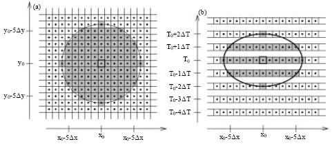 | |
| Fig. 1: | Schematic diagram of spatio-temporal neighborhood for grid point (x0,y0) at time T0. Shaded grid points belong to the neighborhood. (a): The spatial neighborhood in (x,y)-plane. (b): The spatio-temporal neighborhood in (x,t)-plane (adapted from Theis et al. (2005) |
Stated differently, precipitation forecasts at neighboring grid points are considered independent of each other and are assumed to be distributed according to the probability density function for precipitation at point (x0,y0) and time T0. For simplicity, the shape and size of each neighborhood is considered fixed for all times and locations in the entire domain. The forecasts at neighboring grid points are used to calculate the probability of precipitation exceeding a specified threshold. The probability at (x0,y0,T0) is simply the number of grid points in the neighborhood for which the precipitation is forecasted to exceed the threshold, divided by the total number of grid points in the neighborhood. The idea of using an approach based on the neighborhood of each point for quantitative precipitation forecasting is not new. In some newer procedures for precipitation forecast verification, a number of scores has been introduced that rely on spatial patterns of precipitation instead of the value of precipitation intensity at single grid points. A simple verification method that uses the concept of neighborhood was introduced by Atger (2001). In this method, the amount of precipitation in the vicinity of an observation is used to obtain probabilistic forecasts from a single run.
The principal of postprocessing procedure is based on combining two terms (Theis et al. (2005)):
| • | Spatio-temporal distribution of deterministic precipitation forecast |
| • | Probabilistic precipitation forecast for a specified point in space and time |
Both terms express probability, but the two have slightly different meanings. The first term can be used for predictions such as: It will rain tomorrow over 20% of the area and time period of interest and the second statement could be used to make predictions such as: it will rain on 20% of the days like tomorrow.
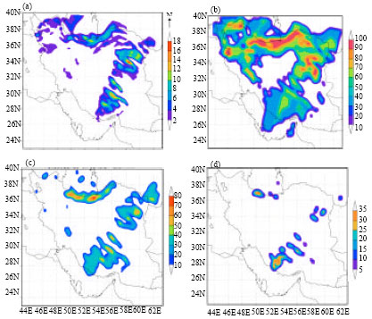 | |
| Fig. 2: | Six hour accumulated precipitation forecast for the 11th of January 2005, 06:00 UTC. (a) Direct model output, (b) Probabilistic forecast for exceedance threshold 1 mm, (c) Probabilistic forecast for exceedance threshold 5 mm and (d) Probabilistic forecast for exceedance threshold 10 mm |
Sometimes these two concepts are confused. Although, these two statements for expressing probability are not the same, we consider the spatio-temporal distribution of precipitation to be a useful estimate of the probabilistic precipitation forecast for a given point in space and time.
Samples of Postprocessing Forecasts
The postprocessing method is implemented on the outputs of the MM5 modeling system using a double nested domain with horizontal resolutions of 45 and 15 km. The inner nest (15 km grid distance) has 242x292 grid points in the horizontal directions and covers the Iran region. Figure 2 shows the 12 h forecast for 6 h accumulated precipitation ending at 06:00 UTC January 11, 2005 and the calculated probabilistic forecasts for different precipitation thresholds for the same date.
Verification
Verification Data
The data gathered from 191 synoptic stations around the country were used to verify the postprocessed forecasts, resulting in a ratio of observation stations to grid points of 1:370. The verification process consisted of comparing each direct observation with the predicted precipitation at the nearest point in the grid. The verification period was from 9 January 2005 to 11 January 2005, during which time significant precipitation was measured at a number of points around the country.
Both the direct output of the model and the probabilistic postprocessed forecast data were compared with observed data. Forecasts' range was considered between 6-24 h. Three different configurations were considered for the spatio-temporal neighborhood, as presented in Table 1.
Verification Measures
Brier Score (BS)
The Brier Score is essentially the mean squared error of the probabilistic forecasts and is defined as the average of the differences between the forecasted probability and the corresponding binary observation:
where, yk is the forecast probability and ok is the corresponding binary observation, assuming that ok = 1 if the observed precipitation exceeds an established threshold, while ok = 0 if it does not and k is the index number of the forecast/event pair. According to the above equation, BS would have a value of zero for a perfect forecast.
Although, BS is a verification measure for the probabilistic forecasts, it can also be used to evaluate deterministic precipitation forecasts based on the direct model output. By setting an exceedance threshold, the precipitation forecast can simply be converted into a dichotomous forecast. A positive sign indicates that the forecast is higher than the threshold value with 100% probability, while a negative sign indicates that the forecast will exceed the threshold value with a 0% probability.
| Table 1: | Different neighborhood configurations for postprocessing |
 | |
Brier Skill Score (BSS)
By considering a reference forecast, the Brier skill score measures the percentage of improvement in the forecast over the reference forecast, as characterized by the measure of accuracy (BS). The BSS values for probabilistic forecasts are given by the following equation (Wilks, 2006; Jolliffe and Stephenson, 2003):
where, the direct model output is used as the reference forecast, thus the BSS shows the percentage improvement of the probabilistic forecast over the direct model output.
Using an algebraic decomposition of the BS (Murphy, 1993), it can be expressed in terms of reliability, resolution and uncertainty:
| (1) |
Relative Value (RV)
The economic value of weather forecasts is frequently dealt with in analytical decision making models (Murphy, 1977). A decision-maker/data user has several options and the option selected is partly influenced by weather forecasts. Any decision has some associated expense that, depending on the circumstances, may result in an economic benefit or loss. The decision-maker's goal is to minimize the expected loss by selecting the optimal option on the basis of all available information. A brief discussion for the economic value of meteorological forecasting, based on the static cost-loss model of Richardson (2000), is presented below:
Consider a user who is sensitive to a climatic event. Assume that the loss to be sustained is L if the event occurs and the user has not taken any protective action, but that he must pay cost C in order to take protective actions. The forecast value is then the net savings to the user, if any, as a result of making use of the forecast. Thus, the forecast will have some positive economic value if it can decrease the user’s total costs when used (Eforecast) in comparison to the costs incurred by a user that has access to the climate forecast (Eclimate) only. The relative value of the forecast is defined by the following equation:
where, Eclimate is calculated as the following:
where, S is the climatological relative frequency of the event or a fraction of the days in which the event happens.
If the forecast is dichotomous, its corresponding contingency table (Table 2) can be used to evaluate the forecast value in the following way:
| Table 2: | Contingency table for dichotomous forecast |
 | |
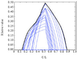 | |
| Fig. 3: | Relative value of probabilistic forecast for 12 h cumulative precipitation. Thin curves are economic value as a function of cost/loss ratio for different probability thresholds and the solid curve is the curve of optimal value |
where, n is the total number of the forecast/event pairs.
To estimate (Eclimate), we assumed that the climatological rate of the event’s occurrence was equal to the rate of the event’s occurrence in the sample. Using this assumption, it can easily be shown that the relative value for a forecast based on climatological information only can be written as:
| (2) |
Where:
 |
False alarm rate measures what fraction of the observed no events were incorrectly forecasted as yes. Hit rate answers the question what fraction of the observed yes events were correctly forecasted. Both scores range from 0 to 1 with value of 1 for a perfect forecast. For a more complete description of these scores see Jolliffe and Stephenson (2003).
If the forecast is probabilistic, the user should consider a threshold probability, Pt, at or above which to take protective actions. RV graphs can be constructed for probabilistic forecasts in terms of α and using different threshold probabilities, with the total area enclosed by these graphs representing the optimal RV value (Jolliffe and Stephenson, 2003). Figure 3 shows relative value of a probabilistic forecast as a function of cost/loss ratio for different probability thresholds and the curve of optimal value.
RESULTS
Verification Results
BSS
In Fig. 4, the BSS for probabilistic forecasts (PPPF) has been plotted for a range of precipitation thresholds, using the direct output of the model (DMO) as the reference forecast. Figure have been plotted for 12 and 6 h cumulative precipitation and in each case, three different configurations have been used for the spatial and temporal neighborhood. As can be seen, the BBS value was positive for all threshold values considered, showing an improvement for the probabilistic forecasts when compared with the corresponding direct model outputs in all cases. Also, it can be seen from the figure that the amount of improvement increases slightly as the size of the neighborhood increases.
The results of decomposing the BS into resolution, reliability and uncertainty parameters (Eq. 1) are shown for the DMO and the postprocessed forecast in Fig. 5. As shown in the Figures, the probabilistic forecast is substantially superior to the corresponding deterministic forecast for both forecast ranges considered, both in terms of reliability and resolution. In the other words, the improvement in the BS score is accompanied by improvements in forecast reliability and resolution. It can also be seen that for higher thresholds, reliability, resolution and uncertainty all decrease due to the decreased event frequency at higher thresholds.
In the postprocessing procedure, the correlation between the forecast probability and the conditional probability of a forecasted event occurring increases as forecast reliability improves.
 | |
| Fig. 4: | Brier skill score of the probabilistic forecast using the direct model output (DMO) as the reference forecast for different configurations; (a) 6 h cumulative precipitation forecast and (b) 12 h cumulative precipitation forecast |
 | |
| Fig. 5: | Reliability, resolution and uncertainty of 6 h cumulative precipitation forecasts for PPPF and DMO, for different configurations |
Relative Value (RV)
In order to calculate relative value statistics, forecasts must first be converted into a dichotomous form, then used to build a corresponding contingency table. From this contingency table, the RV (Eq. 2) can be evaluated as a function of the (C/L) ratio for deterministic and probabilistic forecasts. For the probabilistic forecast, the RV graph for various threshold probabilities is plotted and the curve circumscribing all of these individual RV curves corresponds to the desired optimal curve.
Figure 6 shows the relative value of the PPPF and DMO for 6 and 12 h accumulated precipitation and for 0.1 and 1 mm exceedance thresholds using the largest neighborhood (Table 1). Among the three configurations for the size of neighborhood (Table 1), the largest neighborhood gives the best result in terms of relative value. It is evident from Fig. 6 that the best value is achieved when users select the never protect and always protect options irrespective of the forecast for small (near zero) and large (near one) values of C/L, respectively. The user may make his decision using the forecast only when RV is positive.
In brief, the probabilistic forecast value is higher than the deterministic forecast for all values of C/L and at all precipitation thresholds. Additionally, the postprocessing procedure widens the range of cost/loss ratios in which RV is positive. In other words, more users can make greater use of the forecast when the PPPF approach is used. Considering Eq. 2 for RV with dichotomous forecasts, the maximum RV is always realized by users whose C/L ratio is equal to the climatological rate of event occurrence.
 | |
| Fig. 6: | (a-d) Relative value for DMO (dashed line) and PPPF (solid line) for 12 and 6 h cumulative precipitation forecasts. Upper figures: exceedance threshold of 0.1 mm. Lower figures: exceedance threshold of 1 m |
DISCUSSION
The Goodness of Postprocessed Forecasts
Three criteria for forecast goodness are used: consistency, quality and value (Murphy, 1993). It has been shown that the postprocessed forecast (PPPF) is superior to the deterministic forecast in all three areas.
Forecast Consistency
Since, MM5 is a deterministic model, its output does not contain any information about the uncertainty. A consistent forecast is a forecast that corresponds to an experienced forecaster’s best judgment-thus, if a forecast reflects the uncertainty inherent in the forecaster’s judgment, it would be considered to be consistent in this respect. The main advantage of the postprocessing technique described and implemented here is enhancing the deterministic forecast by including a reasonable level of uncertainty. A postprocessed forecast is thus likely to be nearer to an experienced forecaster’s judgment and, consequently, more consistent than its deterministic counterpart.
Forecast Quality
The forecast quality is related to the degree of correlation between the forecast and empirical observations. BS is a measure used to evaluate forecast quality, while BSS is the corresponding skill score. A review of BSS scores indicates that PPPFs generally produces forecast of greater quality than DMOs. This difference is evident in the increased reliability and resolution obtained using the former approach.
The deterministic forecast does have an advantage over probabilistic forecasts in the area of sharpness, however, since deterministic forecasts always present outcome values of 0 and 100%. However, if these DMO results do not correspond to observed outcomes, the sharpness will be of no practical use.
Forecast Value
The forecast value is a measure of the costs incurred by a user who relies on the forecast to make decisions. As a measure of the forecast value, RV is estimated as a function of the C/L ratio.
For most C/L values, the PPPF is of greater relative value than the DMO. Thus, we can conclude that probabilistic forecasts obtained using a postprocessing procedure typically have greater economic value than deterministic forecasts. The variety of forecasts available to different users with various needs is one of the greatest advantages of the PPPF approach.
It is notable that method for obtaining probabilistic forecast values described in this work includes a kind of calibration process that relies on observation. This calibration is incorporated into the process of selecting the optimal threshold probabilityby maximizing RV. This process is not possible operationally. The obtained results indicate the potential value of the forecast system if the forecast is thoroughly calibrated. Such a well-calibrated probabilistic forecast can divorce the forecaster's and the decision-maker’s roles, unlike the deterministic forecast, in which the forecaster must take on decision-making responsibilities. Close collaboration between forecast providers and users may increase the potential of probabilistic forecasts to effectively meet the needs of users.
The method presented here is adopted to produce probability precipitation forecasts over Iran and the results have been examined using standard verification methods.
CONCLUSIONS
The method applied here for postprocessing is based upon the assumption that precipitation patterns in a given spatio-temporal neighborhood are unpredictable and entirely due to noise. The neighborhood size defines the universal spatio-temporal scale in a way that creates a hypothetical separation between predictable and unpredictable scales. Some corrections can be made to the neighborhood size in order to take into consideration parameters that are independent of the forecast but are correlated with precipitation on the small spatial-temporal scale. The height and slope of geographic features are examples of such parameters. The land surface shape and elevation can be used to change the size and shape of the spatial-temporal neighborhood and to correct the model forecast within the neighborhood. Forecasting power changes with forecast age and this can be expressed as the gradual enlargement of neighborhood size with increasing the forecast age. The short verification period used in this study is another potential source of error that could be investigated in future work by increasing the verification period length.
Finally, it should be noted that the method presented is a simple and inexpensive method for obtaining a probabilistic precipitation forecast from a deterministic model and has the benefits of reducing existing operational barriers such as the need for massive calculations in ensemble systems to obtain a probabilistic framework for such computationally intensive forecasts.
REFERENCES
- Applequist, S., G.E. Gahrs, R.L. Pfeffer and X.F. Niu, 2002. Comparison of methodologies for probabilistic quantitative precipitation forecasting. Weather Forecast., 17: 783-799.
CrossRef - Atger, F., 2001. Verification of intense precipitation forecasts from single models and ensemble prediction systems. Nonlin. Proc. Geophys., 8: 401-417.
Direct Link - Bremnes, J.B., 2004. Probabilistic forecasts of precipitation in terms of quantiles using NWP model output. Mon. Wea. Rev., 132: 338-347.
Direct Link - Theis, S.E., A. Hense and U. Damrath, 2005. Probabilistic precipitation forecasts from a deterministic model: A pragmatic approach. Meteorol. Applied, 12: 257-268.
CrossRef