
A. Ghandhari
Khorasan Razavi Regional Water Authority, Mashhad, Iran
S. M.R. Alavi Moghaddam
Department of Civil Engineer, Islamic Azad University of Mashhad, Mashhad, Iran
Journal of Environmental Science and Technology
Year: 2011 | Volume: 4 | Issue: 5 | Page No.: 465-479


ABSTRACT
Originally, water balance models were introduced to evaluate the importance of different hydrologic parameters under a variety of hydrologic conditions but its present applications are the most common studies at water resources management. In spite of the simple concept of water balance equation, specific considerations are need to proper application. With numerous affecting factors on hydrologic processes, the parsimony trait of water balance equation can cause huge errors or complexities throughout study processes. It is beyond a general computation to create an appropriate portrait of water circumstances with a parsimonious equation that should be considered as an art. Practically, water balance computations are used in five separate categories at least: watersheds, groundwater aquifers, farms, urban water distribution networks and particular areas such as glaciers and landfills; totally, they are directed along three main lines: watershed hydrology reconstruction, evaluation of water supply and water demand systems and assessment of climatic changes impacts. This study is to concentrate on some specific hints which their ignorance leads us to less reliability on water balance results and misunderstandings of actual situations. Finally, the methods used in Iran are investigated in five separate watersheds in the north east of the country and their results are compared with two other published results.
PDF Abstract XML References Citation
Received: January 09, 2011;
Accepted: March 21, 2011;
Published: June 07, 2011
How to cite this article
A. Ghandhari and S. M.R. Alavi Moghaddam, 2011. Water Balance Principles: A Review of Studies on Five Watersheds in Iran. Journal of Environmental Science and Technology, 4: 465-479.
DOI: 10.3923/jest.2011.465.479
URL: https://scialert.net/abstract/?doi=jest.2011.465.479
DOI: 10.3923/jest.2011.465.479
URL: https://scialert.net/abstract/?doi=jest.2011.465.479
INTRODUCTION
Water balance is the base of management and policy making in some critical matters related to water resources management such as design of water supply systems, flood estimation, water allocation and use, management of stormwater and wastewater in urban areas, aquatic ecosystems management, water trading and virtual water. In all of these fields, the basin managers and policy makers need to extract information about the volumes of resources, demands and storage changes in the basin. Based on the results of water balance computations a great number of important water projects have been planed and constructed such as CHASM project in Britain (Quinn et al., 2000) and Doosti complex projects between Iran and Turkmenistan (storage dam, water pipeline to Mashhad city, Sarakhs irrigation network and etc.). Besides, according to the general approach which dominates on water balance concepts, it is a valuable methodology to manage glaciers, snow cover, swamps, estuaries, grasslands, reservoirs and evaluate activities related to water like the effects of mulches on evaporation and evapotranspiration from farms, landfill covers, new instruments effects on nets seepage and etc that have specific analytical conditions (Ghandhari and Ghahraman, 2010;Alkaeed Matsumoto et al., 2004; Nurtayev et al., 2004; Sun et al., 2002; Albright et al., 2004).
The domain of water balance studies can vary from water cycle on the earth to the humidity around a leaf, based on conservation principle. The study targets drive the accuracy rate and the methodology in which computation and application simplicity and reliability are the basses. Because of inherent brevity and parsimony traits of water balance approaches, the water budget models usually focus on prominent aspects of hydrological processes (rainfall-runoff).
The first attempts to develop computer-base models started with SWM (Stanford Watershed Model) in the years between 1959 and 1966 (Crawford and Linsley, 1966; Crawford and Burges, 2004), however, today, numerous models with different assumptions and affecting parameters have been introduced for water balance computations such as: MOSAZ (Modified Semi Arid Zone), AWBM, Sacramento and Curve Number, Makhlouf and Michel, Guo, Wandwiele, Jothityankoon, GR4, PMS, GR2M, VIC-3L, GUI, Wetpass, SESOIL and TOPOG-IRM (Boughton and Chiew, 2007; Boughton, 2004; Mouelhi et al., 2006; Cox and Pitman, 2002; Bonazountas et al., 2005; McCabe and Markstrom, 2007; Abu-Saleem et al., 2010; Najjar, 1999). WASIM (Singh et al., 1999) and WAVES (Mingan et al., 2002) models have specialized for modeling of water balance in a farm. NAM module from MIK-11 is applied to investigate the statistical importance of various parameters in water balance equations (Celleri et al., 2000). It is clear that, the models based on explicit catchment water balance modeling are numbered in the hundreds and new models are still being presented. A major review of water balance models was presented by (Boughton, 2004).
The dominant interests in water balance modeling vary in different countries: Estimation of water yield (Australia), flood estimation (USA) (Boughton, 2004) and budget allocation and putting new constrains on groundwater exploitation (Iran). The wide application of water balance results and decisions which would be made according to them, especially in Iran, show the importance of water balance understanding. The first review of catchment water balance in Iran was done (studied) by Fahmi (1983). This study is an attempt to shed more light on the water balance computation process and its accuracy and also is to present some key points for improving the reliability of water balance results.
PROBLEM DEFINITION
Water balance models have been developed in various time scales (e.g., hourly, daily, monthly and yearly) and different levels of complexity. Monthly water balance models were first developed in 1940s by Thornthwaite and later revised by Thornthwaite and Mather (Xu and Singh, 1998).
At the beginning of computer simulation of catchment water balance, the main purpose was the estimation of runoff for water yield studies and calculated monthly totals of runoff were the main interest. Today, a vast range of models are used in different climates according to the water balance purposes (Xu et al., 1996; Vandewiele and Elias, 1995; Vandewiele et al., 1992; Makhlouf and Michel, 1994; Xiong and Guo, 1999; Legesse et al., 2010). The calculations for monthly totals were made at daily time steps; hence daily runoff values soon became a purpose of calculation. The interest in calculation of daily flows has steadily increased up to the present. However, the use of sub-daily water balance modeling for flood studies is necessary. A good review of monthly water balance models was presented by Xu and Singh (1998) according their applications and kinds of input parameters.
Practical strategies for calculation of dynamic components of water balance equations depend on the targets, accuracy and the time period in which the equations are assessed. In this regard, a lot of internal processes and events are usually neglected and only the response of the region at the end of the period is considered. This property which is called the parsimony, is in the interests of managers due to presenting simplified results. In Iran, it is customary allocating the financial budgets to water resources policies and projects based on the results of water balance analysis between separate regions. So the researchers and engineers are faced with a complicated situation, they should express the complex processes in the form of a simple equation.
However, modeling purposes, target area, calculation method, temporal and spatial boundaries, available data and facilities drive the accuracy of water balance results; generally the degree of accuracy is determined before any computations. Based on the project situations, some important matters such as, choosing an appropriate parent model, avoiding unnecessary details in calculations, using all available data and facilities, model simplification by new scientific achievements and former experiences; should be considered as main directions in the modeling (Ghandhari and Ghahraman, 2009).
The success of the paradigm in relating runoff to rainfall is due to the constraint imposed by the need to account for all water entering, leaving and being stored in a catchment. Complex water balance models that contain error term require correct understanding of backgrounds, feedbacks and interactions between different processes, so more complexity don't necessarily lead us to the more accuracy. Correct modeling key is the match between targets, facilities, available data and model complexity.
Some believe when the time steps of a rainfall-runoff model are selected large enough, the model will be a balance model, in which the ratio of watershed reaction time to the time step is negligible (Mouelhi et al., 2006). Sometimes it can be defined water balance from a simple bucket model to really complex hydrological models according to their resolution (Zhang et al., 2002). In this case, water balance is a set of equations in which each process or a part of process is simulated by an equation. Generally, water budget dominant viewpoints figure out all volumetric components into/out of a three dimensional space that result in storage changes (Burt, 1999). Actually, for achieving to equilibrium between the complexity of model structure and the purposes, we are faced with two sources of errors: systematic errors from simplifier assumptions and calibration errors rising from insufficient or unreliable data that they are inversely related (Zhang et al., 2002).
We can define two separate boundaries and scales for water balance equation: 1-spatial boundaries for the region (spatial scale) and 2-temporal boundary for water balance period (time scale). Selecting different spatial or time scales in a specific region change the accuracy, equation elements and methodology according to the reliability of data, financial conditions and facilities.
Generally, water balance development includes three lumping phenomena; 1-Lumping-spatial basis is related to the averaging of spatial parameters, 2-Lumping-temporal means that accumulative inputs and outputs are considered in a certain period, so intermediate events and their consequences are neglected; however, the scale of the all parameters in a defined model may not be uniform and 3-lumping-conceptual that contains considerations about separate phenomenon in rainfall-runoff processes. Physical point of view may suppose that these assumptions violate the conceptions of modeling; however, the actual modeling results don't approve these judgments. Parameter reduction procedures are general in hydrology to recognition important elements in modeling. These manners use sensitivity analysis to identify parameters with minimum effect on output. One of the general methods is the parameter ratio (Holvoet et al., 2005; Boughton, 2004). Generally, three different techniques can be applied in order to evaluate the parameter significance and sensitivity: (1) Evaluation of the parameter values during the optimization, (2) Checking whether the global minimum is obtained and (3) Detailed analysis of the variance-covariance matrix (Xu and Singh, 1998). The influence of the study scales and the importance of physical characteristics of watershed on water balance equations were studied by surface and subsurface water tracers (Talamba et al., 2000).
Major classifications of water balance computation methods have performed to look at groundwater interactions with surface waters and water use sorts in atmosphere-water-soil system that cause some operational points.
WATER BALANCE IN WATERSHEDS
Water balance is an efficient means for programming and evaluating in the scale of watersheds, applying for water supply and water allocation, waste water management and flood estimation (Anderson et al., 2006; Boughton and Hill, 1997) specially in the case of ungauged basins (Boughton and Chiew, 2007; Boughton, 2004). Long-term water storage changes in watersheds, including surface water and ground water, are expressed in the form of residuals (accumulated or scattered water) in water balance equation (snow and ice amounts can be removed) (Berezovskaya et al., 2005) (Eq. 1):
| (1) |
where, dS/dt is total water change in watershed, P is average precipitation, ET is evapotranspiration and Q is the surface water discharge at the main drain of basin. This simple expression of water balance is valid where the groundwater output and its withdrawals are negligible. Correct definition of water balance period or hydrological year is a very important factor in the simplification of computations and can be evaluated as a basis for judgment about the hydrological regime of watershed (Najjar, 1999).
Classification of watersheds according to homogeneity characteristics (single or multi parametric methods), climate conditions and physiographical situations (closed or open watersheds), can be evaluated as a basis for using the same equations for similar catchments (comparison methods). In closed watersheds, usually, level or volume of the lakes or reservoirs is a controlling factor for evaluating water balance equations (Ghandhari and Ziaii, 2009).
In arid and semi-arid zones, runoff-the basis for calibrating the models as a spatial integration index and controlling factor-is transient and reduce the reliability of results (Mazi et al., 2004). In these zones, it is customary that time series are divided into flooding and non flooding years. It can help to more accuracy in yearly recharge, evaporation and evapotranspiration computations. In flood years, all sub-basins contribute to final discharge that means infiltration, evaporation and evapotranspiration are influenced significantly because of expanded floodplains and vegetation cover development. Loss function is the base for short-time models in arid regions. Dividing a watershed into smaller sub-hydrological systems can improve the results in these basins (Cohen et al., 2001).
Besides, in these kinds of regions, sink areas (AET≥P) are frequently found in, or next to, the stream beds of ephemeral rivers and are often characterized by intensive land use or high conservation values (Ghandhari, 2008). For both types of land use it is important to know if and how much, AET exceeds P and where the lateral water inputs come from. Thick sedimentary fills in the stream bed, variable climate conditions and ephemeral flow conditions pose specific difficulties to the evaluation of the water balance of these sites. Here, the estimated deficit may be compensated by: (a) infiltration of local rainfall during extreme events; (b) runon from the surrounding hill slopes and (c) infiltration of channel flow during flash floods originating from the upper part of the catchment. However, possibilities (a) and (b) cannot explain the water deficit. Deep storage of water during floods in the main channel, can be as much as 60-150 mm per event and may have been 160-400 mm per year in some cases; that is large enough to replenish the annual deficit (Domingo et al., 2001).
A missing component in current water balance models is transmission loss in stream channels between the areas where runoff is generated and the catchment outlet where runoff is measured. The importance of transmission loss is increasing as the importance of low flows for both water allocation and aquatic ecosystems increases.
In some regions, the existence of seasonal ice cover can introduce great deal errors in runoff computations that are why water volume resulted from obstructions and ice resistance causes inefficiency of usual computational techniques (Hamilton, 2004). Accumulation of snow and ice melting and resulted runoff, previous soil moistures, evaporation from intermediate snow, traditional methods for evaporation estimation are the factors affect the results of winter water balances (Kostka et al., 2000).
Precipitation regimes influence the species plants, quality and quantity of their water consumptions, root depth and shading conditions (Comstock and Ehleringer, 1992). Analysis has shown that elderliness is a key factor for trees water consumptions. Old trees near the permanent currents don't use surface water but they transpire from deep layers, so they don't have a significant influenced on surface water balance (Dowson and Ehleringer, 1991). Besides, In some regions, in up to a depth of 1.10 m, shrubs did not compete with crops for water but preferentially extracted water from the lower portion of the profile below 1.10 m and even beyond the depth of 3.5 m (Kizito et al., 2007). However, in arid zones, according to precipitation regimes and plant age, water balance depends on the time of the consumptions among the year (Ehleringer et al., 1991).
Overland flow losses, emerged from evaporation and are really more important than evaporation from open canals. Complexity of interactions between elements of atmosphere-plant-soil system, spatial and temporal variability of vegetation cover, amount of available water and dynamic atmosphere conditions are the agents for complexity of ET computations that take place in the form of water vapor fluxes, a common parameter in water and energy balance equations; that has been identified as a key factor in hydrological modeling. For this reason, several methods have been developed to calculate the potential evapotranspiration (Buttafuoco et al., 2010). It is clear that potential evapotranspiration (ETp) in the standard methods takes place when there is enough moisture in the soil since precipitation is only its source (Najjar, 1999; Kendy et al., 2003). ETp is an essential parameter for computation effective recharge and evaporation from ground water. There are some known methods as Penman-Monteith, FAO56-PM, Thornthwaite and Hargreaves and Hamon to compute ETp. Actually there are not many differences between them, so it seems that FAO56-PM is more suitable for computation of ETp because of its simplicity (Alkaeed et al., 2006). In most of them, air drying power is computed for estimation of ETp and the differences between them refer to the formulating procedure of wind function (Hobbins et al., 2001). Comparison between two common models, AA model (Advection-Aridity) and CRAE model (Complementary Relationship Area Evapotranspiration), shows that CRAE is more powerful means for estimation of regional monthly Etp; however, both of them have present an overestimate values in arid zones. Lidar technique is also a powerful tool to specification and mapping of water vapor on a heterogynous surface (Cooper et al., 2000). Most of the hydrological GIS-based models apply simple interpolation techniques to data measured at few weather stations disregarding topographic effects for Etp. Aguilar et al. (2010) apply a topographic solar radiation algorithm for the generation of detailed time-series solar radiation surfaces using limited data and simple methods in a mountainous watershed in southern Spain. Results show the major role of topography in local values and differences between the topographic approximation and the direct interpolation to measured data (IDW) of up to + 42% and-1800% in the estimated daily values (Aguilar et al., 2010).
To improve the prediction capacity of ETp models for large areas, spatial data should be used as inputs because their continuous variation may reflect more appropriately the nature of the ETp in comparison with the measurements made only at a few weather station locations (Buttafuoco et al., 2010).
GROUNDWATER BUDGET
In watershed budget, usually ground water resources are not investigated as a distinct section but they contribute in equations as a kind of water consumptions (Cohen et al., 2001).
Quantifying noticeable recharges from a vast area due to precipitation, farm irrigations and mountain fronts, especially in arid and semi arid zones is really complicated. Most of the methods that consider the recharge element as a residual component in water balance equations are incorrect because of error margins ranges and inherent uncertainties.
Generally long term groundwater analysis show more desirable results due to the variability of yearly precipitation and volume of irrigation water and not existence appropriate methods to identification of local rising of water table from direct recharges.
Amount of infiltration (recharge) into groundwater depends on vegetation cover and land use, slope and topography, soil composition and hydraulic, water table depth, confining beds presence or totally, soil, vegetation and climatic conditions. There are some known methods which are applied for groundwater budget computations, physical methods such as lysimetry, Water Flux Meters (WFMs) and Tracers (Rockhold et al., 2009) other computational methods like inverse modeling, Richard’s equation solution, tipping-Bucket models and comparison of water table fluctuations in humid and dry periods (Kendy et al., 2003).
As inverse modeling doesn't need to unsaturated zone water movement data, it can be used easily. Although the chemical method and isotropic tracers are very expensive, they are used successfully for quantifying recharge and identifying the sources of feeding in various studies (Rockhold et al., 2009). Richard’s equation solution for vertical flow component in unsaturated zone can be time consuming; besides it needs some difficult measurements such as hydraulic conductivity and soil storage curves but it used successfully to identify and quantify recharge resources. Infiltration storage-routing routine is a suitable method for short time modeling. In this method the downward moisture movement throughout the soil profile is considered providing that moisture is greater than field capacity. Use of this method in large area based on simple 1D model by crop and soil characteristics, meteorological data and hypothesis of independency of successive processes, has showed acceptable results (Kendy et al., 2003).
It is important to know ground water recharge is generally found to be much higher in no vegetated land-use than in vegetated land use (Gee et al., 1994). In the area with fine-grained surficial soils and deep-rooted plants most of the water from direct precipitation is held in the upper 1 or 2 m of the soil column until it returns to the atmosphere by evapotranspiration while deep percolation rates in areas with coarse-grained surficial soils and only shallow rooted plants are greater than in areas with fine grained soils and deep rooted plants (Prych, 1994).
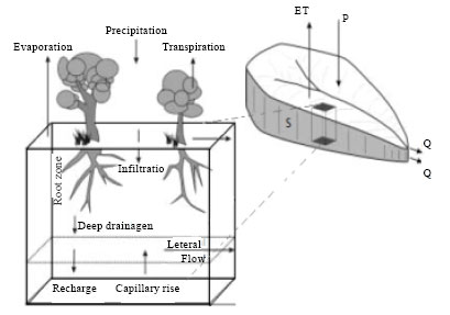 | |
| Fig. 1: | Schematic diagram of water balance for a root zone and a catchment (The box indicates control volume in catchment) |
A suitable control volume to estimate recharge from a farm as a part of a watershed is the root zone in which water balance is referred to unit of area (Fig. 1).
Despite of existence of many methods to compute recharge; hydrological conditions and quantity and quality data determine the desirable method. Appropriate control volume for water balance per unit area and estimating irrigation recharge is root zone. Precipitation can be considered effective on groundwater in two forms: direct infiltration and leakage from runoff (Eq. 2):
| (2) |
where, ΔS is soil water storage change in root zone over the time period, P is precipitation, I is interception losses, ET is evaporation and transpiration totally, RO is overland flow or runoff, DD is deep drainage out of root zone, R is recharge to groundwater and SSF is lateral subsurface flow.
Usually piezometric observations are applied to control the calculations in aquifers. It is very important to consider that the causes of the piezometric levels variations are not only related to the pumping test and water deductions intend to supply towns, agricol and industrial sectors. The geometrical configuration of the aquifer could also play a significant role in the understanding of these variations (Zouhri et al., 2005).
FARM WATER BALANCE
In the farm water balance, the field measurements are not effective alone. They are time consuming noticeably and they cost and don’t obtain continues data; however, usually it is essential to trace different parts of total irrigation water. In farm we usually need to indentifying portion of leaching water and evapotranspiration as a percent of total irrigation water. Therefore, farm water balance models need to develop some modules and codes for evaluation of conveyance budget, root zone moisture and etc. (Zhang, 2002).
Water shortages, water rights, project developments, irrigation system efficiency, common water resources around the farm (as springs) and returned water from adjacent farms are arguments that result in serious legal challenges in many catchments and plains. These challenges have created a basis for a new definition as beneficial or intelligent use of water allocation among different sectors and users, according to water balance approaches (Burt, 1999). In this way it can be define the irrigation efficiency as the ratio of benefitted irrigation water (consumed by crops) to irrigation water minus soil storage increasing (Isidoro et al., 2004). In the case of the farm managements there are a great number of modes as aforementioned.
THE IMPACTS OF HUMAN ACTIVITIES AND CLIMATE CHANGE ON WATER BALANCE
Land cover change, associated with the intensification of agriculture, cattle rising and urbanization, could have a profound influence on the hydrological processes in small watersheds and at a regional level (Mendoza et al., 2010). Developing water balance formulations, especially when the targets contain future programming based on forecasts, significantly depend on human activities and climate change; however, a lot of models have a disability to incorporate these effects.
Human activity has the potential to indirectly and directly affect water quantity and the natural flow regime of a river system. Indirect impacts to the hydrologic cycle can result from land-use changes. Direct impacts can result from water diversions, withdrawals and discharges and from dams (flow regulation and water storage).
Urban and rural developments and followed physical changes in a part of the catchment can have significant quantitative and qualitative effects on streams and currents. All kinds of structures such as roads, fences, asphalted areas and etc can change the natural river regimes and increase accidental hydrological events. In fact, changes to the landscape caused by urban structures development can affect hydrologic systems in two major ways, termed closed circuited and non-closed circuited land use. Closed circuited areas include areas where the impacted land is hydrological isolated from the original drainage area and no longer contributes flow to the river system. Non-closed circuited land change includes areas that still contribute flows to the river systems but where vegetation has been removed or other changes affecting water flow havWatsone occurred. Some artificial surface nets create closed circuited in some processes as flow and pollution conveyances solution and absorption on soil particles, delayed feedback mechanisms, surface maintenance and biological degradations in unsaturated zones.
In small basins, small-scale forest management activities increase total discharge, direct runoff, groundwater recharge and base flows (Bent, 2001). Environmental degradation and native vegetation removals or change the type of the forest trees cause changes in soil compositions and its hydraulic properties (Wahl et al., 2003) and after that changes the situation of ground water recharge components (Zhang et al., 2002).
There are some models such as Macaque model, TOPOG, ANTHROPOG, MM5 and SWAT which have been used effectively to investigate some effects of human activates on local water cycle components (Watson, 1999; Fohrer et al., 2001; Ghandhari and Ghahraman, 2010).
Dam construction with big reservoirs that can store considerably volume of yearly discharges, in some countries such as Iran produced significant effects on watershed water budget and hydrologic conditions (Ghandhari and Ghahraman, 2010).
Climate change can cause significant impacts on water resources through changes in the hydrological cycle. The change in temperature and precipitation components of the cycle can have a direct consequence on the quantity of evapotranspiration and runoff components. Consequently, the water balance can be significantly affected (Legesse et al., 2010). PDO and ENSO are two natural known phenomena affecting water balance parameters. In some countries such as US, climate change has been identified as critical key for water sustainability (Hansen et al., 2004). The water balance models have proven to be a valuable tool not only for assessing the hydrologic characteristics of diverse watersheds but also for evaluating the hydrologic consequences of climatic change. In the last 10 years, monthly water balance models have been used to explore the impact of climatic change (Xu and Singh, 1998). For the purpose of water resources assessment and climate change impact study, a semi distributed monthly water balance model is proposed and developed to simulate and predict the hydrological process and water resources in macro scale basins in China with (Guo et al., 2001).
Use of a physically based hydrological model integrating all hydrological processes on basin scale with GIS and RS technologies, to assist the water balance components simulation, is the best alternative approach for lumped and/or empirical methods (Abu-Saleem et al., 2010), so now-a-days, RS and GIS are considered as two basic elements in hydrological modeling and simulation. Determination of vegetation cover areas and their types, impermeable areas, river and their bank vegetation conditions that show an intermediate status, ET, precipitation properties and snow properties can be determine with RS. Satellite images have more advantages than field images, considering to economic issues and their accuracy; however, satellite images don’t have a lot of restrictions (Goetz and Jantz, 2004; Wenzhong and Youjing, 2009; Berezovskaya et al., 2005; Dewan et al., 2005). In Iran RS can be suppose the best technique because of insufficient appropriate databases and reliable enough data especially about the farms (Ghandhari, 2004). One parameter of special interest for water management applications is the crop coefficient employed by the FAO-56 model to derive actual crop evapotranspiration (ET) by RS radiometric measurements. Combinations RS data with daily soil water balance in the root zone is used to estimate daily evapotranspiration at field scale (Padilla et al., 2010). Besides, precipitation radar data are really useful for distributed surface hydrological processes modeling because of their high resolution and time and space continuity. Guo et al. (2004) prepared an almost complete list of radar data applications until 2004 and they showed NEXRAD data receive precipitation special distribution more effective than rain gages by using their effect on water balance of watershed. Today, there are Mathematical-GIS based algorithms to extract the hydrological features such as drainage networks, ridge networks and watersheds accurately (Dinesh, 2008).
WATER BALANCE EVALUATION STUDIES IN FIVE WATERSHEDS IN THE NORTH EAST OF IRAN
Although, all available information collecting are required for further understanding of the problem aspects, usually objects and parameter estimation methods lead to eliminate some insignificant parameters. Despite of relatively simple conceptual analysis of water balance equations, the number of components, parameter calculation methods and specific local conditions determine the structure and procedures of water balance equations. However, it has been tried to choose the simple method with desirable variability (Ghandhari and Ghahraman, 2009).
Practically, water balance computations are based on expert judgments that are why today there are not enough data and definition data collecting and field measurement as a part of water balance studies in Iran. Usually ET is computed according Thornthwaite method, Darcy’s law is used for water movement in saturated zones and then recharge from farms, plains, urban and rivers estimated as a portion of annual precipitation empirically. Because of these percentages are considered without any data and measuring documents, they are really unreliable. Here five separate watersheds with different hydrological and geological conditions are compared briefly and then the results of a modeling according to a simple form of Richard’s approach (Kendy model) in one of these watersheds and the results of two published studies are investigated (Fig. 2). Comparison shows there are significant deviations between supposal percentages and actual ones (Table 1).
| Table 1: | Study results on separate catchments |
 | |
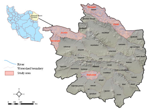 | |
| Fig. 2: | Five catchments in Khorasan Razavi province of Iran |
In a region as Khorasan Razvi province of Iran with 250 mm yearly precipitation, water is the main determinative factor for all activities. It means an error about 7% for 54472 ha, 7% for 104 km river with 0.44 L sec-1 mean discharge and 15% for 7852 M^3 of daily domestic water are significant.
CONCLUSION
Understanding this issue that a lot of common engineering analytic methods (quantitative and qualitative), developed models and softwares which are used for analysis the water problems are based on the water balance equations; can help us to find the best method for modeling.
In some countries such as Iran, most of the models used in water resources planning have been extracted from other countries with different climate conditions. It is very important to concentrate on the basis of these models before using them. Determination of minimum standards, required number of parameters and estimation methods in separate local zones, required reliability, new techniques and tools for reducing costs, field measurements and so on; can help to achieve more effective water management. Already developed methods that are the base for strategic decision making and financial budget allocations don’t have reliable basis.
REFERENCES
- Albright, W.H., C.H. Benson, G.W. Gee, A.C. Roesler and T. Abichou et al., 2004. Field water balance of landfill final covers. J. Environ. Qual., 33: 2317-2332.
PubMed - Anderson, R., J. Hansen, K. Kukuk and B. Powell, 2006. Development of a watershed-based water balance tool for water supply alternative evaluations. Proceedings of the Water Environment Federation, (WEF`06), Water Environment Federation, pp: 2817-2830.
CrossRef - Berezovskaya, S., D. Yang and L. Hinzman, 2005. Long term annual water balance analysis of the Lena River. Global Planetary Change, 48: 84-95.
CrossRef - Bonazountas, M., D. Panagoulia, N. Passas, K. Syrios and G. Grammatiko, 2005. Water balance estimation via soil: Pinios river basin, Greece. Ball. Eng. Geol. Environ., 64: 111-116.
CrossRef - Boughton, W., 2004. Catchment water balance modelling in Australia 1960-2004. Agric. Water Manage., 71: 91-116.
Direct Link - Boughton, W. and F. Chiew, 2007. Estimating runoff in ungauged catchments from rainfall, PET and the AWBM model. Environ. Modell. Software, 22: 476-487.
CrossRef - Burt, C.M., 1999. Irrigation water balance fundamentals. Proceeding of the Conference on Benchmarking Irrigation System Performance using Water Measurement and Water Balance, March 1999, San luis Obispo, CA. USCID, Denever, Colo, pp: 1-13.
Direct Link - Celleri, R., L. Timbe, R.F. Vazquez and J. Feyen, 2000. Assessment of the relation between the NAM rainfall-runoff model parameters and the physical catchment properties. Proceedings of the Conference on Monitoring and Modeling Catchment Water Quantity and Quality, Sept. 27-29, Ghent, Belgium, pp: 9-16.
- Cohen, M.J., C. Henges-Jeck and G. Castillo-Moreno, 2001. A preliminary water balance for the Colorado River delta, 1992-1998. J. Arid Environ., 49: 35-48.
Direct Link - Comstock, J.P. and J.R. Ehleringer, 1992. Plant adaptation in the great basin and Colorado plateau. Great Basin Nat., 52: 195-215.
Direct Link - Cooper, D.I., W.E. Eichinger, J. Kao, L. Hippes and J. Reisner et al., 2000. Spatial and temporal properties of water vapor and latent energy flux over a riparian canopy. Agricult. Forest Meteorol., 105: 161-183.
CrossRef - Cox, J.W. and A. Pitman, 2002. The Water Balance of Pastures in a South Australian Catchment with Sloping Texture-Contrast Soils. In: Regional Water and Soil Assessment for Managing Sustainable Agriculture in China and Australia, McVicar, T.R., L. Rui, J. Walker, R.W. Fitzpatrick and L. Changming (Eds.). ACIAR Monograph Canberra, Australia, pp: 82-94.
- Crawford, N.H. and S.J. Burges, 2004. History of the stanford watershed model. Water Resources IMPACT, Vol. 6.
Direct Link - Dowson, T.E. and J.R. Ehleringer, 1991. Streamside trees that do not use stream water. Nature, 350: 335-337.
CrossRef - Ehleringer, J.R., S.L. Philips, W.S.F. Schuster and D.R. Sandquist, 1991. Differential utilization of summer rains by desert plants. Oecologia, 88: 430-434.
Direct Link - Fohrer, N., S. Haverkamp, K. Eckhardt and H.G. Frede, 2001. Hydrologic response to land use changes on the catchment scale. Phys. Chemi. Earth Hydrol. Oceans Atmos., 26: 577-582.
CrossRef - Goetz, S.J. and C.A. Jantz, 2004. Integrated analysis of ecosystem interactions with land use change: The chesapeake bay watershed. Ecosyst. Land Use Change Geophys. Monograph Series, 153: 263-275.
Direct Link - Guo, J., X. Liang, L.R. Leung, 2004. Impacts of different precipitation data sources on water budgets. J. Hydrol., 298: 311-334.
CrossRef - Hobbins, M.T., J.A. Ramirez and T.C. Brown, 2001. The complementary relationship in estimation of regional evapotranspiration: An enhanced Advection-Aridity model. Water Resou. Res., 37: 1389-1403.
Direct Link - Holvoet, K., A.V. Griensven, P. Seuntjens and P.A. Vanrolleghem, 2005. Sensitivity analysis for hydrology and pesticide supply towards the river in SWAT. Phys. Chem. Earth, 30: 518-526.
CrossRef - Isidoro, D., D. Quilez and R. Aragues, 2004. Water balance and irrigation performance analysis: La Violada irrigation district (Spain) as a case study. Agr. Water Manage., 64: 123-142.
CrossRef - Kendy, E., P. Gerard-Marchant, M.T. Walter, Y. Zhang, C. Liu and T.S. Steenhuis, 2003. A soil-water-balance approach to quantify groundwater recharge from irrigated cropland in the North China Plain. Hydrol. Process., 17: 2011-2031.
CrossRef - Makhlouf, Z. and C. Michel, 1994. A two-parameter monthly water balance model for French watersheds. J. Hydrol., 162: 299-318.
CrossRef - Matsumoto, T., R. Naruse, K. Konya, S. Yamaguchi, T. Yamada and Y.D. Muravyev, 2004. Summer water balance characteristics of koryto Glacier, Kamchatka Peninsula, Russia. Geografiska Annaler Phys. Geography, 86: 181-190.
Direct Link - Mazi, K., A.D. Koussis, P.J. Restrepo and Koutsoyiannis, 2004. A ground water-based objective heuristic parameter optimization method for a precipitation-runoff modl and its application to a semi-arid basin. J. Hydrol., 290: 243-258.
CrossRef - Mouelhi, S., C. Michel, C. Perrin and V. Andreassian, 2006. Stepwise development of a two-parameter monthly water balance model. J. Hydrol., 20: 1-15.
CrossRef - Najjar, R.G., 1999. The water balance of the Susquehanna River Basin and its response to climate change. J. Hydrol., 219: 7-19.
CrossRefDirect Link - Nurtayev, A.N.B., M. Petrov, A. Tikhanovskaya and I. Tomashevskaya, 2004. The share of a glacial feeding in water balance of Aral Sea and Karakul Lake. J. Marine Syst., 47: 143-146.
CrossRefDirect Link - Singh, P., G. Alagarswamy, P. Pathak, S.P. Wani, G. Hoogenboomb and S.M. Virman, 1999. Soybean-chickpea rotation on Vertic Inceptisols I. Effect of soil depth and landform on light interception, water balance and crop yields. Field Crops Res., 63: 225-236.
CrossRef - Quinn, P.F., P.E. O'Connell, C.G. Kilsby, G. Parkin and M.S. Riley et al., 2000. Catchment hydrology and sustainable management (CHASM): Generic experimental design. Proceedings of the Conference on Monitoring and Modeling Catchment Water Quantity and Quality, (MMCWQQ`00), Ghent (Belgium), pp: 77-81.
- Sun, G., S.G. McNulty, D.M. Amatya, R.W. Skaggs, L.W. Swift, J.P. Shepard and H. Riekerk, 2002. A comparison of the watershed hydrology of coastal forested wetlands and the mountainous uplands in the Southern US. J. Hydrol., 263: 92-104.
CrossRef - Vandewiele, G.L. and A. Elias, 1995. Monthly water balance of ungauged catchments obtained by geographical regionalization. J. Hydrol., 170: 277-291.
CrossRef - Vandewiele, G.L., C.Y. Xu and N.L. Win, 1992. Methodology and comparative study of monthly water balance models in Belgium, China and Burma. J. Hydrol., 134: 315-347.
CrossRef - Wahl, N.A., O. Bens, B. Schafer and R.F. Hutt, 2003. Impact of changes in land-use management on soil hydraulic properties: Hydraulic conductivity, water repellency and water retention. Phys. Chem. Earth Parts A/B/C, 28: 1377-1387.
CrossRefDirect Link - Xiong, L. and S. Guo, 1999. A two-parameter monthly water balance model and its application. J. Hydrol., 216: 111-123.
CrossRef - Xu, C.Y., J. Seibert and S. Halldin, 1996. Regional water balance modelling in the NOPEX area: Development and application of monthly water balance models. J. Hydrol., 180: 211-236.
CrossRef - Zhang, L., G.R. Walker and W.R. Dawes, 2002. Water Balance Modelling: Concepts and Applications. In: Regional Water and Soil Assessment for Managing Sustainable Agriculture in China and Australia, McVicar, T.R., L. Rui, J. Walker, R.W. Fitzpatrick and L. Changming (Eds.). ACIAR Monograph Canberra, Australia, pp: 31-47.
- Xu, C.Y. and V.P. Singh, 1998. A review on monthly water balance models for water resources investigations. Water Resour. Manage., 12: 20-50.
CrossRef - Zhang, X., 2002. Linking water balance to irrigation scheduling: A case study in the piedmont of Mount Taihang. In: Regional Water and Soil Assessment for Managing Sustainable Agriculture in China and Australia, McVicar, T.R., L. Rui, J. Walker, R.W. Fitzpatrick and L. Changming (Eds.). ACIAR Monograph Canberra, Australia, pp: 57-69.
- Abu-Saleem, A., Y. Al-Zubi, O. Rimawi, J. Al-Zubi and N. Alouran, 2010. Estimation of water balance components in the hasa basin with GIS based wetspass model. J. Agron., 9: 119-125.
CrossRefDirect Link - Gee, G.W., P.J. Wierenga, B.J. Andraski, M.H. Young, M.J. Fayer and M.L. Rockhold, 1994. Variations in water balance and recharge potential at three western desert sites. Soil Sci. Soc. Am. J., 58: 63-72.
CrossRefDirect Link - Dinesh, S., 2008. Extraction of hydrological features from digital elevation models using morphological thinning. Asian J. Scientific Res., 1: 310-323.
CrossRefDirect Link - Zouhri, L., B.B. Kabbour, C. Gorini, B. Louche, J. Mania, B. Deffontaines and M. Dakki, 2005. The hydrodynamism of the coastal aquifer system belonging to the Southern border of the rharb basin (Morocco). J. Applied Sci., 5: 678-685.
CrossRefDirect Link - Dewan, A.M., K. Kankam-Yeboah and M. Nishigaki, 2005. Assessing flood hazard in greater dhaka, Bangladesh using SAR imageries with GIS. J. Applied Sci., 5: 702-707.
CrossRefDirect Link - Legesse, D., T.A. Abiye, C. Vallet-Coulomb and H. Abate, 2010. Streamflow sensitivity to climate and land cover changes: Meki River, Ethiopia. Hydrol. Earth Syst. Sci., 14: 2277-2287.
CrossRef - Buttafuoco, G., T. Caloiero and R. Coscarelli, 2010. Spatial uncertainty assessment in modelling reference evapotranspiration at regional scale. Hydrol. Earth Syst. Sci., 14: 2319-2327.
CrossRef - Aguilar, C., J. Herrero and M.J. Polo, 2010. Topographic effects on solar radiation distribution in mountainous watersheds and their influence on reference evapotranspiration estimates at watershed scale. Hydrol. Earth Syst. Sci., 14: 2479-2494.
CrossRef - Kizito, F., M. Sene, M.I. Dragila, A. Lufafa and I. Diedhiou et al., 2007. Soil water balance of annual crop-native shrub systems in Senegal's Peanut Basin: The missing link. Agric. Water Manage., 90: 137-148.
CrossRef - Hansen, R.T., M.W. Newhouse and M.D. Dettinger 2004. A methodology to asess relations between climatic variability and variations in hydrologic time series in the Southwestern United States. J. Hydrol., 287: 252-269.
CrossRef - Mendoza, M.E., G. Bocco, E. Lopez-Granados and M.B. Espinoza, 2010. Hydrological implications of land use and land cover change: Spatial analytical approach at regional scale in the closed basin of the Cuitzeo Lake, Michoacan, Mexico. Singapore J. Trop. Geogr., 31: 197-214.
CrossRef
kuol malual nyok ayak Reply
i need sample of hydro logic cycles models