
M.A. Dong
School of Humanities and Social Science, Harbin Institute of Technology, Harbin City, 150001, People`s Republic of China
Journal of Applied Sciences
Year: 2014 | Volume: 14 | Issue: 9 | Page No.: 932-937


ABSTRACT
This study focuses on the fact that traditional supply chain management method is harder to adapt to the uncertainty or randomness of such a dynamic complex system. Two supply chain models are constructed under different production strategies of make to stock and build to order. Dynamical character of supply chain as complex system such as bifurcation and chaos under certain conditions are analyzed by the calculating the models’ Lyapunov Index, power spectrum and correlation dimension. The feasibilities of flexible production of manufacturer groups, together with the reasons and countermeasures of bull-whip effect in supply chain, are discussed by utilizing chaotic ergodicity and sensitivity of initial conditions.
PDF Abstract XML References Citation
Received: December 26, 2013;
Accepted: February 10, 2014;
Published: March 22, 2014
How to cite this article
M.A. Dong, 2014. Research on Supply Chain Models and its Dynamical Character Based on Complex System View. Journal of Applied Sciences, 14: 932-937.
DOI: 10.3923/jas.2014.932.937
URL: https://scialert.net/abstract/?doi=jas.2014.932.937
DOI: 10.3923/jas.2014.932.937
URL: https://scialert.net/abstract/?doi=jas.2014.932.937
INTRODUCTION
The aim of supply chain management is to form an integrated network system through the organic connections of plan, production, distribution and storage, sale and service and other activities, thus, to save cost and improve economic performance. Wang et al. (2012) argued that the nodes and complex supply and demand relationships among the nodes and all exchanges with systems beyond supply chain and surroundings enables the supply chain system is complicated and supply chain management is also complex. Therefore, from and only from complexity, it is possible to reveal the internal rule for optimization of supply chain system. The complexity in studies of supply chain management with system dynamics and simulation technique aroused great attention in information, control and management field.
With the development of supply chain management and increasing academic attention to complex systems approach, the research achievements of supply chain based on complex systems are growing. Choi et al. (2001) first put forward that complex adaptive system can be used in the research of supply chain and meanwhile emphasizes the necessity of regarding the supply chain as a complex adaptive system. Laumanns and Lefeber (2006) argued bullwhip effect of supply chain is connected with its network topology. Kuhnert et al. (2006) found that the material supply system of the city to the scale-free distribution. Laumanns and Lefeber (2006) established a directed supply chain network to realize the goal of supply chain by robust optical control. Pathak et al.(2007) pointed out the usefulness of researching supply chain management integrating with the theory of complex system. Guo (2006) conducted a series of research on the directed output of the supply chain, proposed the G model and calculated the degree distributions and stationary average degree distributions of the network model by using the renewal process theory and the continuum theory and shows that the supply chain networks have bilateral power-law distributions. Gao et al. (2011) established a preferential attachment model to describe the evolution of supply chain by analyzing its node’s production, decline and deletion. Yu et al. (2009) suggested that the weighted network evolution theory can be introduced into the supplychain system and formed complex system evolving model of supply chain based on trading quantity. Song (2010) built refined oil complex system of supply chain through the empirical research based on the trading quantity. Barabasi and Albert (1999) assumed that nodes and the time internal entered the system and the arrival time of nodes followed the uniform distribution in the course of the BA model analysis and argued their deficiency of their BA model analysis, which showed that the assumption of nodes, time interval entering system in BA model can’t reflect the real situation of the supply chain network growth. According to the above analysis, we found that the studies on the application of complex system in economy management, especially in supply chain management are relatively insufficient. The deficiency of existing research is mainly manifested in the following two aspects:
| • | There is too much emphasis on the complex theory of physics, which can’t reflect the characteristics of supply chain, such as Helbing et al. (2006) research on bullwhip effect |
| • | Taking the supply chain systems under the different production strategies as the same complex system ignored their different dynamic characteristics of the system |
But all those studies are centered on individual problems in supply chain system, which lack of witnesses for complexity of supply chain system and nonlinear characteristics and application. This study builds two supply chain models under two different production strategies. Dynamic characteristics of supply chain as complex system such as bifurcation and chaos under certain conditions are analyzed by the calculating the models’ Lyapunov Index, power spectrum and correlation dimension. The evolution of the situation is emulated and an economic explanation is presented. Based on theses, a new supply chain management model is put forward.
SUPPLY CHAIN MODEL UNDER DIFFERENT PRODUCTION STRATEGIES
The theoretical framework of supply chain model is the foundation to build system model and its optimization, control and other analyzing work.
Supply chain features on several aspects: complexity is one compared with individual enterprise; dynamical character is shown on supplying, manufacturing, marketing and material flow, capital flow and information flow; demand-oriented character is the drive source of material flow, capital flow and information flow (Yu et al., 2012). For convenience, the research explores the three-level supply chain system consisted of customer-dealer-manufacturer and puts forward a hypothesis based on above features.
Hypothesis 1: The sales volume of a product t+1 rests with customers’ possession and consumption quantity of the products during stage t, i.e., potential customers are driven by conformity. With the increase of sales volume, the market saturation of the product increases and thus restrains its further sailing, described by the following mathematical equation:
| (1) |
where, xt+1 is the demand quantity at stage t+1 (when xt+1<0, customers’ rejection or disgust can be described); yt is the possession quantity at stage t (i.e., production quantity at stage t); k stands for the degree of influence the possession quantity of customers on potential customers; k1 (k1≥0) is capacity of the market; k2 (0≤k2≤1) is market saturation.
Hypothesis 2: During the transmission of customer’s demand information from dealer to manufacturer, there is one unit time delay, i.e., the demand information dealt with by manufacturer at stage t+1 is the information at stage t. The delay results in information distortion. The decision makers on every node of supply chain usually process the demand information they get and result in further information delay and distortion. If it is reasonable, it can be described by mathematical equation as the following:
| (2) |
Here yt+1 is production quantity at stage t+1 (when yt+1<0, it reflects the virtual production quantity resulted from customers’ disgust for the product). Because of the delay of information, it can only be manufactured according to demand quantity at stage t. k3 is information distortion due to delay of demand information; when k3≤0, it means demand quantity is magnified for manufacturers; when k3≥0, it means demand quantity shrinks.
Production strategy mainly contains make to stock (abbreviated as MTS) (Sun et al., 2005) and build to order (abbreviated as BTO). MTS refers to make production plan and procurement plan according to customer’s demand and safety stock; BTO refers to make production directly according to customer’s demand and without taking safety stock into consideration. Combined the above two hypothesis, two dynamical models of supply chain system are built:
| • | Supply chain model under MTS: |
| (3) |
Here k4 (0≤k4≤1) is coefficient of safety stock
| • | Supply chain model under BTO: |
| (4) |
All the following supply chain models are models under MTS except special instructions. The supply chain system under BTO has similar conclusions with proven results. Unnecessary details are not given here.
DYNAMICAL CHARACTER OF SUPPLY CHAIN MODEL
In Eq. 3, when parameter values are k1 = 1.5, k2 = 0.3, k3 = 2.1, k4 = 0.1, x1 (0) = 0.6, y1 (0) = 0.6, by MATLAB simulation, x-y phase diagram of supply chain system can be got as Fig. 1.
Through research on Lyapunov exponent, power spectrum and correlation dimension, further studies can be made to reveal its dynamical nature.
Lyapunov exponent: Lyapunov exponent is an index of the quantitative description of the diverging nature of adjacent tracks in phase space. If Lyapunov exponent is negative, it means the volume of phase space shrinks with stabilized movement and being not sensitive to initial value; if Lyapunov exponent is zero, then it corresponds with critical state, i.e., a stable boundary, if Lyapunov exponent is positive, it means adjacent tracks moves divergently and be very sensitive to initial value and in chaos.
There are many algorithms to calculate Lyapunov exponent. This study adopts Gram-Schmidt orthogonal technology algorithm (Gao et al., 2011).
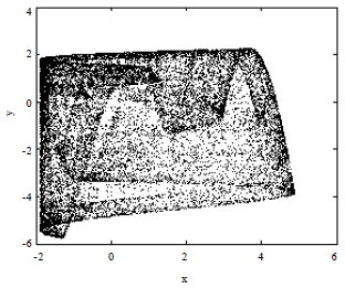 | |
| Fig. 1: | X-y phase diagram |
Detailed process is as follows:
| • | Suppose an autonomous system flows through x0 space and forms an orbit x (t). If the initial conditions x0 have deviation Δx0, then from x0+Δx0, another orbit forms. Therefore, another tangent space vector Δx (x0, t) forms and definition deflection ratio is w (x0, t) = Δx (x0, t). To choose a fixed tiny time interval τ and calculate wk-1 (τ) by wk-1 (0), to go from x((k-1)τ) to x(kτ), firstly the following equation can be got: |
| (5) |
| (6) |
Here j = 1, 2, …, 0, orthogonal algorithm is used:
| (7) |
| (8) |
| (9) |
Based on high order and first order relationships, No. p first order Lyapunov exponent can be got:
| (10) |
Equation 10 is the algorithm of Lyapunov exponent.
Under these parameters and with the above algorithm, Lyapunov exponent spectrum of the chaotic time series in system 3 can be calculated as 0.158115 and 0.078138, i.e., the Lyapunov exponent spectrum with interference is (+, +) type. The corresponding evolution of time series in Lyapunov exponent is as Fig. 2.
Obviously with time going on, time series in Lyapunnov exponent is always above zero, which indicates the system is in chaos.
Power spectrum: Chaotic motion features on aperiodic motion and complexity and distinguishes itself from divergent nature in periodic motion or quasi-periodic motion.
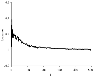 | |
| Fig. 2: | Lyapunov exponent of system |
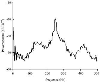 | |
| Fig. 3: | Power spectrum of system |
It is continuous spectrum. The algorithm is to calculate the average time of sample function Fourier transform squared, i.e.:
| (11) |
For time series x0 , x1, …, xN-1 (the time increment is Δt), Fourier transform is:
| (12) |
| (13) |
where, pk is time window. With Fourier transform FFT, X (jw) can be got.
Figure 3 is power spectrum of system (3) under the above parameters. The continuity of power spectrum peak can be found and the system is in typical chaotic state at present.
Bifurcation: Bifurcation vividly explains the geometrical nature of chaotic time series, i.e., there are similarities between the part and the whole on structure, form and function. When the observation scale changes, similarities do no change at all, the complexity and irregular shape of bifurcation by quantitative description with correlations dimension cam be done. It can stand for the degree of influence from nature, state and amount of variables of supply chain system. It also can be used to distinguish chaotic nature of supply chain and predict future changes in production decision making. Taking C-C algorithm, the embedded dimension 15 of chaotic time series can be got and time delay is τ = 3. The algorithm of correlations dimension designed by Grassberger-Procaccian is as follows.
To embed time series into multi-dimensional phase space and to connect phase point is to present the evolution tracks of the system in re-constructed phase space. The correlations can be estimated by Euclidean distance. The equation of Euclidean distance is as follows:
| (14) |
Suppose one number r, then to check the number of distances between other points to this number r and it is shown like d (rI, rj)<r. The correlation integral C (r) stands for the proportion of distances shorter than r from points to r in all distances Nm (Nm-1), thus the next formula can be got:
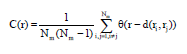 | (15) |
In Eq. 15, θ (x) is step function, i.e.:
| (16) |
To choose a proper section r, then there is the following relations between C (r) and r:
| (17) |
Then, D is the correlations dimension of the wanted time series and the following equation can be got:
| (18) |
In actual calculation, after choosing a section of r, many C(r) can be got. With the slope of In C(r) and In r straight line regression, correlation dimension D is gotten. After increasing embedded dimension m, when D begins to be stable with m increase, the D at this point is the correlation dimension in wanted time series.
With the above methods, the relationships of InC (r)~In r when the variables of system 3 between the embedded dimension 5, 6 and 7 (m = 1) are as it is shown in Fig. 4. Based on the above, correlations dimension is 1.79664, which indicates that the system is a complex and chaotic one.
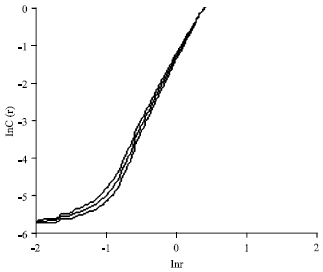 | |
| Fig. 4: | Correlation dimension of system |
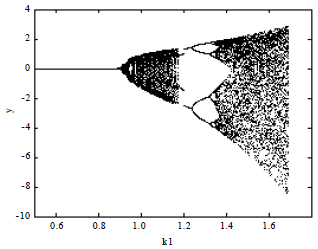 | |
| Fig. 5: | Evolutionary figure of production quantity decision changed with k1 |
Simulation of the evolution of the supply chain system: From the above analysis, system 3 shows such complex characters within some parameters random as bifurcation and chaos that the nonlinear system has. When parameter k1 changes constantly within [0, 1.8], i.e., consumption demand volume changes within a fixed section but the other parameters keep stable, the evolution of manufacturer’s production strategy is as Fig. 5 shows. It shows that the system changes into monocyclic, divergent and chaotic state. This is due to the increasing demand of customers. Initially manufacturers can employ new staff, purchase raw materials and equipment thus to meet consumption demand and to keep the monocyclic state of demand and distribution proportion being balanced within the enterprise. But the capital is limited. When supply cannot meet demand, the two separate with each other. With the deviation of the two is being bigger, finally chaos is resulted in. At this moment, the production is still not random. It still changes with demand volume, the attracting factor. If the enterprise again matches its production capacity with consumption demand through self-organizations like reconstruction and mergers and acquisitions, it can jump out of chaos and start a new cycle. The evolution continues without ending and finally goes into chaos.
Chaos is a pseudorandom process of seemingly irregular motion. It is predictable in short period but unpredictable in a long period. The change of chaos changes with the exchanging of system materials, energy and information with outsider conditions. Nonlinear system can change from simple to complex and according to a fixed way. For example, with period doubling bifurcation phenomenon, self-similarity within supply chain appears and the system goes into chaos. Therefore, the future of the system can be predicted by changing features.
CHAOS AND SUPPLY CHAIN OPERATION
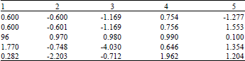
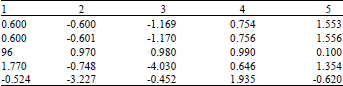
Chaos brings negative influence to the process of supply chain, such as bull-whip effects. Bull-whip effects refer to the magnification of market demand and instability of the system brought by magnification. For example, the stock volume and cost of stocking during supply, manufacture and sale stages all increase; dealer have stock redundancy and manufacturers have over-production; stock volume in supply chains and production strategy are in chaos. This is due to the fact that production strategy sensitivity depends on consumption demand. Any tiny change of consumption demand makes a big deviation of predicted results with time delay. As Table 1 shows, demand information is delayed and distorted during its transmission. Moreover, any tiny change of parameters also results in different results. As Table 2 shows, all can result in the deviation of production quantity of manufacturers and actual market demand. That is bull-whip effect.
Chaos also benefits for supply chain management. For example, manufacturers can make flexible production utilizaing chaotic features. Flexible production refers to the ability for enterprises to deal with internal and external environmental changes. It overcomes the conflicts between specificity of production equipments and diversity of market demand and improves the competence of enterprises. Under monocyclic conditions, when market demand waves greatly, the cost of transformation between different production states is comparatively high, such as the change of staff, raw material, purchasing or selling production equipments and so on.
| Table 1: | Title difference of production decisions changes caused by the changes of consumption demand x1 |
 | |
| Table 2: | Difference of production decisions changes caused by the changes of k3 |
 | |
When the system is in doubling period or chaos, due to the ergodicity of chaos and its sensitivity to initial conditions, when chaos evolutes close to target state, with the most tiny interference, such as slight change of some parameter, after a temporary state, the system will be stable at the target state. Thus with a tiny cost, the transformation of different production states is finished and the simply transformation is impossible for a non-chaotic system.
In real practice, man need to organize flexible production with chaotic features of supply chain and prevent the negative effects of chaos. Because of supply chain system is not always in chaos. Whether chaos appears and when it appears are under conditions. Therefore, it is feasible to control chaos according to different demand. Changing parameters or initial conditions of the system, on one hand, can motivate bifurcation and induce the system into chaos and make flexible production; on the other hand, can restrain bifurcation and eliminate or delay chaos and take control of chaos.
CONCLUSION
This study puts forward supply chain model under MTS and BTO strategies based on complex, dynamical, user-oriented and interlocking character of the system. The study also analyses such nonlinear characters of the supply chain system as bifurcation and chaos under certain conditions through calculation of Lyapunov exponent, power spectrum and correlation dimension. The supply chain system produces bull-whip effect at chaotic state, which can be restraint by short-period prediction and fasten the transmission of demand information and other methods. Chaos also shows benefits to enterprises. For example, it makes low-cost flexible production possible, which is of high theoretical and practical value. However, at present there is little research on this. It could be the next research target of supply chain management.
REFERENCES
- Wang, J. and X. Wang, 2012. Complex dynamic behaviors of constrained supply chain systems. Syst. Eng. Theory Pract., 32: 746-751.
Direct Link - Choi, T.Y., K.J. Dooley and M. Rungtusanatham, 2001. Supply networks and complex adaptive systems: Control versus emergence. J. Oper. Manage., 19: 351-366.
CrossRefDirect Link - Helbing, D., D. Armbruster, A.S. Mikhailov and E. Lefeber, 2006. Information and material flows in complex networks. Phys. A Stat. Mech. Appl., 363: 11-16.
CrossRefDirect Link - Kuhnert, C., D. Helbing and G.B. West, 2006. Scaling laws in urban supply networks. Phys. A Stat. Mech. Appl., 363: 96-103.
CrossRef - Laumanns, M. and E. Lefeber, 2006. Robust optimal control of material flows in demand-driven supply networks. Phys. A Stat. Mech. Appl., 363: 24-31.
CrossRef - Pathak, S.D., J.M. Day, A. Nair, W.J. Sawaya and M.M. Kristal, 2007. Complexity and adaptivity in supply networks: Building supply network theory using a complex adaptive systems perspective. Decis. Sci., 38: 547-580.
CrossRef - Guo, J.L., 2006. The bilateral Power-law distribution model of supply chain networks. Acta Physica Sinica, 55: 3916-3921.
Direct Link - Gao, L., J.L. Guo and H.Y. Jia, 2011. Supply chain model with deletion mechanism. Commer. Res., 1: 43-47.
Direct Link - Yu, H., L. Zhao and X. Lai, 2009. Trade Quantity-based supply chains networks evolving model. Chinese J. Manage., 2: 187-191.
Direct Link - Song, S., 2010. The empirical research of refined oil supply chain weighted network on complex theory. Technol. Market, 17: 36-40.
Direct Link - Barabasi, A.L. and R. Albert, 1999. Emergence of scaling in random networks. Science, 286: 509-512.
CrossRefDirect Link - Yu, J., S. Ma and Q. Zhou, 2012. Comparative study of supply chain coordination based on MOI and VMI under random yield and uncertain demand. Chinese J. Manage. Sci., 20: 64-74.
Direct Link