Classification of Images for Automatic Textual Annotation: A Review of Techniques

MATERIALS AND METHODS

In this experiment, WEKA was chosen as a tool for performing image classification. Features from the collected image are extracted and represented as WEKA data representation. A few learning algorithms were chosen which was reported to perform relatively better than other algorithms, particularly for small training set.

WEKA: WEKA (Hall et al., 2009) was used to evaluate the performance of image classifiers. WEKA is an open source java based machine learning tool. WEKA provides various learning algorithms namely under the categories; bayes, functions, lazy, meta, mi, misc, rules and trees. All available algorithms were compared and a few were chosen for more detailed evaluation based on the most performed and liaised with a few work done by other researchers. The classification task is to predict the class of images whether being ‘beach’, ‘building’, ‘festival’ or ‘mountain’.

Image feature extraction: Colour feature is one of the most widely used feature in Image Retrieval. Colour Histogram is the most used in colour feature representation (Rahman, 2002; Kaushik et al., 2012). Colour histogram performs well especially when images have mostly uniform colour distribution (Kodituwakku and Selvarajah, 2004). 3D Colour Histogram is used to extract image feature. Each pixel in the image is projected into a 3D RGB colour space. 3D colour space is divided into 4x4x4 and 6x6x6 cells which generates colour histogram with 64 bins and 216 bins, respectively. The number of pixels in each cell are counted and stored in the colour histogram. The histogram is normalized by summing up the total number of pixels in each bin and dividing each value by the total value. The normalized data gives the proportion of pixels as a percentage for each bin.

Learning algorithms: In this experiment, a number of representative machine learning algorithms were evaluated namely, SVM, Multilayer Perceptron, Bagging, DECORATE, C4.5 Decision Tree and Random Forest. Initially, all available algorithms in WEKA were compared and these few were chosen for more detailed evaluation based on the most performed and liaised with a few work done by other researchers. The following are brief description of these algorithms.

Support vector machine: A Support Vector Machine (SVM) is a supervised learning method that analyzes data and recognizes patterns, employed for classification and regression analysis. SVM uses kernels to transform the linearly non-separable data in one domain into another domain where the instances become linearly separable. Kernel equations may be linear, quadratic, Gaussian, or anything else that accomplishes the aforementioned purpose.

Once the data is separated into two distinct categories, the best hyper-plane dividing the two types of instances is identified. Future prediction is dependent on this hyper-plane in deciding the target variable value. A hyper-plane that is chosen should be one that maximizes the margin between the support vectors on either side of the plane. Support vectors are those instances that are either on the separating planes on each side, or a little on the wrong side.

SVM handles binary data (two-class data) that is separable by a linear classifier. Even if the data is not binary, SVM treats it as though it is and analyses completely through a series of binary assessments on the data. In a multi-class classification, SVM applies the one-against-one approach by fitting all binary subclassifiers and finding the correct class by a voting mechanism.

Multilayer perceptron: A Multilayer perceptron (MLP) is a feedforward neural network, having one or more layers between input and output. It maps sets of input data onto a set of suitable output. Feedforward manner means that data flows in one direction, that is, from input to output layer. An MLP has multiple layers of nodes in a directed graph, where each layer is fully connected to the subsequent one but with exception for the input nodes. Each node is a neuron with a nonlinear activation function. MLP is trained using the backpropagation supervised learning technique. MLP is a modification of the standard linear perceptron, which can distinguish data that is not linearly separable (Cybenko, 1989).

The activation function of each neuron is modeled in several ways, but should at all times be normalizable and differentiable. The two main activation functions used in current applications are described by the following equation:

where, y_i is the output of the ith node (neuron) and v_i is the weighted sum of the input synapses. The former function is a hyperbolic tangent ranging from -1 to 1 and the latter, the logistic function, ranges from 0 to 1 but is similar in shape.

Bagging: Bootstrap aggregating (bagging) is a machine learning ensemble meta-algorithm to improve machine learning of statistical classification and regression models in terms of stability and classification accuracy (Breiman, 1996). It lessens variance and aid to steer away from overfitting. Bagging can be applied with any type of model, even though it is commonly applied to decision tree models. It is a special case of the model averaging technique.

Given a standard training set D of size n, bagging generates m new training sets D_i, each of size n'>n, by sampling examples from D uniformly and with replacement. By sampling with replacement, it is probable that some examples will be repeated in each D_i. If n' = n, then for large n the set D_i is expected to have, on average, 63.2% of the unique examples of D, the rest are duplicates appearing multiple times.

DECORATE: DECORATE is a meta-learner for building diverse ensembles of classifiers by using specially constructed artificial training examples (Melville and Mooney, 2003). In DECORATE, an ensemble is generated iteratively. It first learns a classifier and then adding it to the current ensemble. At the beginning, the ensemble contains the classifier trained on the given training data. Subsequently, at each successive iteration, the classifiers are trained on the original training data combined with artificial data. Artificial training examples are generated from the data distribution in each iteration. The number of examples to be generated is specified as a fraction, R_size, of the training set size. The labels for these artificially generated training examples are chosen in a way to be different, as much as possible, from the current ensemble's predictions. The labelled artificially generated training data is known as the diversity data. A new classifier combining the original training data and the diversity data are trained and thus resulting in a diverse ensemble. By adding this classifier to the current ensemble would increase its diversity. While forcing diversity, the training accuracy still need to be conserved. Thus, a new classifier is rejected if it was found that by adding it to the existing ensemble decreases its accuracy. This process is repeated until the required committee size is attained or the maximum number of iterations is surpassed.

The following is the method used to classify an unlabeled example, x. Each base classifier, C_i, in the ensemble C* yields probabilities for the class membership of x. If P_Ci,y(x) is the estimated probability of example x belonging to class y according to the classifier C_i, then the class membership probabilities is computed for the entire ensemble as:

where, P_y(x) is the probability of x belonging to class y. The most probable class is selected as the label for x, i.e., C*(x) = arg max_yεYP_y(x).

C4.5 Decision tree: C4.5 is an algorithm used to generate a decision tree (Quinlan, 1993). C4.5 is often referred to as a statistical classifier as the decision trees generated by C4.5 can be applied for classification.

To classify a new item, the following method is employed. C4.5 first creates a decision tree based on the attribute values of the existing training data. Each time it comes across a set of items (training set) it identifies the attribute that discriminates the various instances most distinctively. The feature that can describe the data instances, maximally, to enable classifying them the best is said to have the highest information gain. Among the possible values of this feature, if data instances falling within its category have the same value for the target variable, then that branch is terminated and assigned to it the target value that was obtained.

On the contrary, if there is ambiguity, another attribute that has the highest information gain is considered. This is continued until either a clear decision of what combination of attributes gives a particular target value, or it runs out of attributes. If it was the case that it runs out of attributes, or if it cannot get an unambiguous result from the existing information, this branch is assigned a target value that the majority of the items under this branch possess.

With the decision tree, the order of attribute selection is followed as it was obtained for the tree. By checking all the respective attributes and their values with those seen in the decision tree model, the target value of this new instance is able to be predicted.

Random forest: Random forests are a combination of tree predictors such that each tree depends on the values of a random vector sampled independently and with the same distribution for all trees in the forest.

Random forests are ensemble classifiers that are a combination of many decision trees in such a way that each tree depends on the values of a random vector sampled independently and with the same distribution for all trees in the forest. The method combines Breiman's "bagging" idea and the random selection of features, in order to construct a collection of decision trees with controlled variation (Breiman, 2001).

Each tree is formed using the following algorithm:

For classification, a new item is pushed down the tree. It is assigned the label of the training sample in the terminal node it ends up in. This is iterated on all trees in the ensemble and the average vote of all trees is concluded as random forest prediction.

Performance metrics: Nine performance metrics were used to compare the aforementioned learning algorithms. Correctly classified instances is the number of images that are correctly classified. Time taken, on the other hand is the total amount of time taken to complete classification process of an algorithm. The kappa statistic measures the agreement of prediction with the true class, 1 signifies complete agreement.

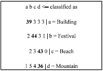
For the rest of the performance metrics, it is best explained with the aid of a confusion matrix. Confusion matrix is more commonly named contingency table. In this study, there are four classes and therefore a 4x4 confusion matrix (as illustrated in Fig. 1). The number of correctly classified instances is the sum of diagonals in the matrix; all others are incorrectly classified. For example, for the class ‘building’ in Fig. 1, it was wrongly classified as ‘festival’ three times and for the class ‘festival’, it was wrongly classified as ‘building’ twice.

The True Positive (TP) rate is the proportion of examples which were classified as class x, among all examples which truly have class x, i.e., how much part of the class was captured. It is equivalent to Recall. In the confusion matrix, this is the diagonal element divided by the sum over the relevant row, i.e., 39/(39+3+3+3) = 0.813 for the class ‘building’ in this example.

The False Positive (FP) rate is the proportion of examples which were classified as class x, but belong to a different class, among all examples which are not of class x. In the matrix, this is the column sum of class x minus the diagonal element, divided by the rows sums of all other classes; i.e., 5/(50+48+46) = 0.035 for the class ‘building’ in the above example.

The Precision is the proportion of the examples which truly have class x among all those which were classified as class x. In the matrix, this is the diagonal element divided by the sum over the relevant column, i.e., 39/(39+2+2+1) = 0.886 for the class ‘building’.

Fig. 1:	An example of a confusion matrix

The F-Measure is simply a combined measure for precision and recall as represented by the following equation:

Accuracy is measured by the area under the ROC curve. The area under the ROC curve measures the discriminating ability of a binary classification model. An area of 1.00 represents a perfect test; an area of 0.5 represents a worthless test. A rough guide for classifying the accuracy of a diagnostic test is the traditional academic point system as follows:

These measures are useful for comparing classifiers.

Dataset: The algorithms were compared using a dataset consisting of 429 images from the Flickr Tourism Malaysia which have four classes, namely, ‘beach’, ‘building’, ‘festival’ and ‘mountain’. Images that are chosen specifically under the category of Tourism Malaysia is intentionally done to aid subsequent work of image annotation. Images were divided into two groups; one is the training images and the other, is the testing images. Feature extraction that acts as attribute which are evaluated by the classifiers is provided in Attribute-Relation File Format (ARFF).

RESULTS AND DISCUSSION

The image data set were divided into two categories, i.e. set A and B. Set A represents 192 images chosen, having strong distinctive feature amongst classes. Set B, on the other hand, represents images possessing 237 less distinctive feature amongst classes. Comparative results are shown on corrected classified instances which is measured by percentage, time taken to produce results, kappa statistics, false positive, precision, recall, F-Measure, ROC Area and accuracy.

Table 1-6 show the classification performance for various learning algorithms. Image classification in Table 1-3 uses 3D Colour Histogram feature extraction with 64 bins. Whereas classification in Table 4-6 uses 216 bins.

Results for classification using the same training and testing images from set A with 64 bins is as shown in Table 1. Both DECORATE and Random Forest produces 100% accuracy, but the number of correctly classified instances for Random Forest is slightly lower. The result is consistently the same when taking set B as the training and testing images, as shown in Table 2.

However, when taking set A as the training set and set B as the testing set (as shown in Table 3), Bagging shot right up to top the rest. Bagging showed better performance with an accuracy of 72.8%, slightly outperforming DECORATE by 0.7%. A specific experiment was carried out by Pal (2007) to evaluate the effect of noise on the classification performance using four different ensemble approaches; bagging, DECORATE, random subspace and boosting. The fact that bagging is able to handle dataset with noise the best, as reported by Pal (2007), may be a contributing factor to the results.

Table 4 shows the scores for classification using the same training and testing images from set A with 216 bins. Both DECORATE and Random Forest produces 100% accuracy, but the number of correctly classified instances for DECORATE is slightly lower. When taking set B as the training and testing images, as shown in Table 5, DECORATE and Random Forest scored 100% accuracy and 100% correctly classified instances.

The scores for classification of set A as training set and set B as testing set with 216 bins is as shown in Table 6. DECORATE showed the best performance with 87.6% accuracy. This is followed by Bagging and Random Forest with 86.8% accuracy.

Overall, DECORATE has shown the best performance. In terms of time taken, Random Forest seems to be the quickest and Multilayer Perceptron being the slowest.

Table 1:	Results for classification using the same training and testing images from set A with 64 bins

Table 2:	Results for classification using the same training and testing images from set B with 64 bins

Table 3:	Results for classification of set A as training set and set B as testing set with 64 bins

Table 4:	Scores for classification using the same training and testing images from set A with 216 bins

Table 5:	Scores for classification using the same training and testing images from set A with 216 bins

Table 6:	Scores for classification of set A as training set and set B as testing set with 216 bins

Different number of bins can reveal different features of data. In this experiment, representing image features as 216 bins performed better than the 64 bins. The results show that all learning algorithms performed best with 216 bins with an increased accuracy between 7.4-16.1% as compared to the 64 bins.

The result presented indicates the potential performance of DECORATE in classifying images especially involving small training set. The best overall performance shown by DECORATE is consistent to Melville and Mooney (2003) where they reported that DECORATE is consistently more accurate than the base classifier of Bagging, AdaBoost and Random Forests. But given large training sets, DECORATE is still competitive with AdaBoost and outperform Bagging and Random Forests.

Another experiment carried out by Caruana and Niculescu-Mizil (2006) reported that Random Forest perform about 0.6% better than the next best method, ANN. This is followed by boosted decision trees and SVMs. These results are in line with ours where Random Forest has outperformed decision trees and SVM. The aforementioned experiment however did not include DECORATE.

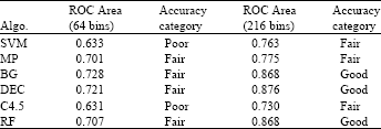
Table 7:	Classification

Due to the high effectiveness and reliability of using multi-class SVM in image classification as reported by previous researchers, SVM was chosen without any specific experiments done (Molitorisova, 2012; Lindstaedt et al., 2009; Khan 2007; Cusano et al., 2003). Nonetheless, this study concluded that other classification algorithms perform better than SVM.

Table 7 shows the accuracy category for the various classifiers based on the area under the ROC curve. It clearly shows that the DECORATE, Random Forest and Bagging model achieved ‘good’ discriminating ability as compared to other classifiers. However, DECORATE has slightly higher ROC area as compared to the Random Forest and Bagging classifier.

CONCLUSION

This study has shown, via classification, that certain high-level semantic categories can be learnt using specific low-level image features. It has distinguished classes ‘beach’, ‘building’, ‘festival’ and ‘mountain’. DECORATE has shown the best performance on the whole, followed closely by Random Forest and Bagging. Despite that classification performance rely on the algorithm of the classifier itself, the accuracy of the classifiers also depends on the features used, since the features are inputs that act as attributes to the classifiers. The performance improved when feature 3D Colour Histogram with 64 bins were replaced by 216 bins. The number of training samples, on the other hand, influences the classifier’s ability to learn the true decision boundary from the training data. Such a classification is important for the task of image annotation as the idea to group similar images into the same semantic category. A near future work is to explore methods for assigning suitable tags or annotation to new images based upon previously tagged similar images.

It is assumed that images that are visually similar to the target image, will suggest good annotation to it. The suggested annotation will be merged, refined and enhanced to produce the final annotation.

REFERENCES

- Caruana, R. and A. Niculescu-Mizil, 2006. An empirical comparison of supervised learning algorithms. Proceedings of the 23rd International Conference on Machine Learning, June 25-29, 2006, Pittsburgh, PA., USA., pp: 161-168.
CrossRef - Caruana, R., N. Karampatziakis and A. Yessenalina, 2008. An empirical evaluation of supervised learning in high dimensions. Proceedings of the 25th International Conference on Machine Learning, July 5-9, 2008, Helsinki, Finland, pp: 96-103.
CrossRef - Cybenko, G., 1989. Approximation by superpositions of a sigmoidal function. Mathe Control Signals Syst., 2: 303-314.
CrossRefDirect Link - Fan, J., Y. Gao and H. Luo, 2008. Integrating concept ontology and multitask learning to achieve more effective classifier training for multilevel image annotation. IEEE Trans. Image Process., 17: 407-426.
CrossRef - Hall, M., E. Frank, G. Holmes, B. Pfahringer, P. Reutemann and I.H. Witten, 2009. The WEKA data mining software: An update. SIGKDD Explorat. Newslett, 11: 10-18.
CrossRefDirect Link - Kaushik, M., R. Sharma and A. Vidhyarthi, 2012. Analysis of spatial features in CBIR system. Int. J. Comput. Appli., 54: 11-15.
CrossRefDirect Link - Khan, L., 2007. Standards for image annotation using Semantic Web. Comput. Stand. Interfaces, 29: 196-204.
CrossRef - King, R., C. Feng and A. Shutherland, 1995. Statlog: Comparison of classification algorithms on large real-world problems. Applied Artif. Intell.: Int. J., 9: 289-333.
CrossRef - Kodituwakku, S.R. and S. Selvarajah, 2004. Comparison of color features for image retrieval. Indian J. Comp. Sci. Eng., 1: 207-211.
Direct Link - Lindstaedt, S., R. Morzinger, R. Sorschag, V. Pammer and G. Thallinger, 2009. Automatic image annotation using visual content and folksonomies. Multimed. Tools Appli., 42: 97-113.
CrossRef - Melville, P. and R.J. Mooney, 2003. Constructing diverse classifier ensembles using artificial training examples. Proceedings of the 18th International Joint Conference on Artificial Intelligence, August 9-15, 2003, Acapulco, Mexico, pp: 505-510.
Direct Link - Noah, S.A. and D.A. Ali, 2010. The role of lexical ontology in expanding the semantic textual content of on-line news images. Proceedings of the 6th Asia Information Retrieval Societies Conference, December 1-3, 2010, Taipei, Taiwan, pp: 193-202.
CrossRef - Pal, M., 2007. Ensemble learning with decision tree for remote sensing classification. World Acad. Sci. Eng. Technol., 12: 258-260.
Direct Link - Shi, R., C.H. Lee and T.S. Chua, 2007. Enhancing image annotation by integrating concept ontology and text-based bayesian learning model. Proceedings of the 15th International Conference on Multimedia, September 23-28, 2007, Augsburg, Bavaria, Germany, Pages: 341-344.