
Saowapha Chaipitak
School of Applied Statistics, National Institute of Development Administration, Bangkapi District, Bangkok, 10240, Thailand
Samruam Chongcharoen
School of Applied Statistics, National Institute of Development Administration, Bangkapi District, Bangkok, 10240, Thailand
Journal of Applied Sciences
Year: 2013 | Volume: 13 | Issue: 2 | Page No.: 270-277


ABSTRACT
This study proposed a test for the equality of two covariance matrices from two independent multivariate normal populations with high-dimensional data. The test statistic is based on unbiased and consistent estimator of the ratio between the sums of squares of covariance matrix elements. Under the null hypothesis, the proposed test statistic is asymptotically standard normal distributed when the number of variables and the sample sizes go together to infinity. Simulation study is conducted to investigate the performance of the proposed test statistic. The results showed that the proposed test is superior to the other three tests appeared in the literature for various patterns of common covariance matrix. Finally, two real data sets are analyzed to illustrate the application of our theoretical results.
PDF Abstract XML References Citation
Received: October 18, 2012;
Accepted: December 19, 2012;
Published: February 21, 2013
How to cite this article
Saowapha Chaipitak and Samruam Chongcharoen, 2013. A Test for Testing the Equality of Two Covariance Matrices for High-dimensional Data. Journal of Applied Sciences, 13: 270-277.
DOI: 10.3923/jas.2013.270.277
URL: https://scialert.net/abstract/?doi=jas.2013.270.277
DOI: 10.3923/jas.2013.270.277
URL: https://scialert.net/abstract/?doi=jas.2013.270.277
INTRODUCTION
Let xij = (xij1, ..., xijp)’, j = 1, ..., ni, i = 1,2, be random samples drawn from independent multivariate normal populations Np(μi, Σi), where all the parameters are unknown. It is a requirement in many statistical techniques, such as in discriminant analysis, testing the equality of two mean vectors, testing the equality of two mean sub-vectors, to know whether covariance matrices of the two populations are equal or not (Johnson, 1998; Krzanowski, 2000; Srivastava, 2002; Gamage and Mathew, 2008; Fujikoshi et al., 2010). Before applying any further analysis, this equality must be tested. The widely used traditional technique for testing the hypothesis that H0: Σ1 = Σ2 = Σ against H1: Σ1≠Σ2 where Σ is the common unknown covariance matrix of the two populations, when the sample sizes ni larger than the number of variables, p, is the modified likelihood ratio test. However, in applications concerning modern sciences and economics, the data consist of very large number of variables taken from small samples. For instance, DNA microarrays typically measure thousands to millions of gene expressions on the small sample sizes (Dudoit et al., 2002; Ibrahim et al., 2002; Sebastiani et al., 2006; Huang et al., 2009). When the data have p≥ni, called high-dimensional data, the sample covariance matrices Si are singular making the modified likelihood ratio test is not valid. The tests under this problem were recently worked by Schott (2007), Srivastava (2007) and Srivastava and Yanagihara (2010). To have more powerful choice of test statistic for testing H0 against H1 when p≥ni, a new test statistic is proposed. It is shown that this proposed test statistic is asymptotically distributed as the standard normal distribution for any type of common covariance matrix considered with large p, ni.
Let ni be the sample size drawn from population i, i = 1, 2 and n = n1+n2-2, the following assumptions are made:
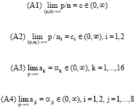 |
where, ak = (trΣk)/p and aji = (trΣji)/p.
Let:
 |
and
| (1) |
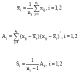
Since S1 and S2 are independent estimates of the covariance matrices Σ1 and Σ2, respectively, with (ni-1) Si ∼Wp (Σi, ni-1), i = 1, 2, where Wp (Σi, ni-1) is a Wishart distribution with ni-1 degree of freedom and covariance matrix Σi then the common covariance matrix Σ can be estimated by:
Let:
and
| (2) |
The modified likelihood ratio test suggested by Bartlett (1937) on an intuitive ground is based on the statistic:
and is valid when p<ni. In particularly, if p is fixed, the asymptotic null distribution of -2 log L, as ni→∞, for i = 1, 2, is chi-squared distribution with p(p+1)/2 degree of freedom.
Because of the unavailability of the modified likelihood ratio test L when p≥ni, Schott (2007) proposed a test for the equality of several covariance matrices. This study then considers Schott’s test statistic only for the case of two covariance matrices. Based on the consistent estimator of the square of Frobenius norm of Σ1-Σ2, namely tr(Σ1-Σ2)2 his test statistic is given by:
Under the null hypothesis, TJ is asymptotically distributed as N (0, 1) as (p, n1, n2)→∞.
Srivastava (2007) proposed a test based on a lower bound on Frobenius norm. It is given by:
where:
and
where, c0 = n (n3+6n2+21n+18), c1 = 2n (2n2+6n+9), c2 = 2n (3n+2) and c3 = n (2n2+5n+7). Under the null hypothesis TS is asymptotically distributed as N (0, 1) as (p, n)→∞.
Srivastava and Yanagihara (2010) proposed an alternative test based on a consistent estimator of a measure of distance by ![]() , where
, where ![]() , i = 1, 2. The consistent estimators of γi are given by
, i = 1, 2. The consistent estimators of γi are given by ![]() . The test statistic is given by:
. The test statistic is given by:
where:
and
Under the null hypothesis, TSY is asymptotically distributed as N (0, 1) as (p, n)→∞.
THE PROPOSED STATISTIC
To test the hypothesis H0: Σ1 = Σ2 = Σ against H1: Σ1≠Σ2 for p≥ni it is observed that if Σ1 = Σ2, then ![]() . Thus under the null hypothesis, the measurement
. Thus under the null hypothesis, the measurement ![]() . Using lemma A3 extended from lemma A1 obtained from Srivastava (2005) in the Appendix, a consistent estimator of b can be estimated by
. Using lemma A3 extended from lemma A1 obtained from Srivastava (2005) in the Appendix, a consistent estimator of b can be estimated by ![]() . The following lemma gives the asymptotic distribution of the consistent estimators.
. The following lemma gives the asymptotic distribution of the consistent estimators.
Lemma 1: Let (ni-1) Si∼Wp (Σi, ni-1), â2i, i = 1, 2, as defined in (1) and ![]() , then under the assumptions (A2) and (A4):
, then under the assumptions (A2) and (A4):
 |
where, ![]() denotes x converges in distribution to y.
denotes x converges in distribution to y.
Proof: Since random samples xij, j = 1, ..., ni, i = 1,2 are drawn from two independent populations and sample covariance matrices Si are calculated from corresponding independent random samples x1j and x2j thus, S1 and S2 must be independent of each other. In fact, the statistic â21 is a function of S1 alone while the statistic â22 is also a function of S2 alone. Thus â21 and â22 are also independent and then it makes COV (â21, â22) = 0. By lemma A4 in the Appendix, â2i, i = 1, 2 are asymptotically normally distributed with mean a2i and variance:
and the fact that the covariance between â21 and â22 is zero, it follows that the jointly asymptotic distribution of statistics â21 and â22 are the bivariate normal distribution with mean vector and covariance matrix as given above. The proof is completed.
Note that ![]() is a ratio of two uncorrelated estimators. By the delta method (Lehmann and Romano, 2005), it ensures that a function of two random variables can be approximated as normal distribution. The following theorem establishes the asymptotic normality of the statistic
is a ratio of two uncorrelated estimators. By the delta method (Lehmann and Romano, 2005), it ensures that a function of two random variables can be approximated as normal distribution. The following theorem establishes the asymptotic normality of the statistic ![]() .
.
Theorem 1: Let b and ![]() be as defined above. Then, under the assumptions (A1)-(A4),
be as defined above. Then, under the assumptions (A1)-(A4), ![]() , where:
, where:
Proof: We note that ![]() . Hence the partial derivative of
. Hence the partial derivative of ![]() with respect to â21 is:
with respect to â21 is:
Similarly, the partial derivative of ![]() with respect to â22 is:
with respect to â22 is:
Thus, by applying the delta method, ![]() asymptotically with:
asymptotically with:
 |
The proof is completed.
Corollary 1: Let ![]() be as defined above. Under H0: Σ1 = Σ2 = Σ and the assumptions (A1)-(A4), then:
be as defined above. Under H0: Σ1 = Σ2 = Σ and the assumptions (A1)-(A4), then:
 |
Proof: Under H0, then a21 = a22 = a2 and a41 = a42 = a4. Thus:
It follows Theorem 1, then the proof is completed.
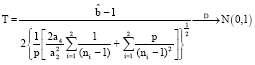
In order to use T in practice, we have to estimate δ2 involving estimate of a2 and a4. Under the null hypothesis and by using consistent estimators of a2 and a4 as â2 and â*4 as given in lemmas A1 and A5 in the Appendix, respectively and by assumption (A2), we obtained a corresponding consistent estimator of δ2 namely ![]() as:
as:
Thus a test of H0 is based on the statistic:
and also its asymptotic null distribution is the standard normal. The proposed test statistic T* with α level of significance rejects H0 if |T*|>zα/2 where zα/2 denotes the upper α/2 quantile of the standard normal distribution.
SIMULATION STUDY
Here, the performance of the proposed test statistic T* compared to three tests TJ, TS and TSY was shown through numerical simulation technique. In order to assess being normality of the tests, the Attained Significance Level (ASL) of these tests were simulated and expected to be close to the nominal significance level setting. The empirical powers of these tests in different situations were also performed.
Parameter selection: Independent 10,000 replications of the multivariate normal random datasets were generated using International Mathematics and Statistics Library (IMSL) with multivariate normal random number generator (RNMVN) subroutine of Fortran programming language (FORTRAN). The nominal significance level α used was 0.05. Under the null hypothesis, the test statistics T*, TJ, TS and TSY were computed and the proportions of rejection of test statistics under the null hypothesis were recorded, called the Attained Significance Level (ASL). In our work presented here, the ASL under the null hypothesis and corresponding empirical power under the alternative hypothesis were manipulated for following hypotheses in different patterns of covariance matrix setup as follow:
| • | Unstructured pattern (UN): It is defined as Σ = (σij)pi,j=1. We considered the hypothesis as follows: | |
| • | ||
| • | ||
| where, U0 = (σij)pi,j=1 where σij = 1 (if i = j); σij = (-1) i+j (0.10i)/j (if i≠ j) and U1 = (σij)pi, j=1 where σij = 1 (if i = j); σij = (-1)i+j (0.05i)/j (if i ≠ j) | ||
| • | Compound Symmetry pattern (CS): It is defined as Σ = σ2Ip+k1p1'p, where σ2>0, k is appropriate constant, Ip denotes the pxp identity matrix and 1p denotes the px1 vector of ones. The hypothesis was set as: | |
| • | ||
| • | ||
| • | Heterogeneous compound symmetry pattern (CSH): It is defined as Σ = (σij)pi,j = 1 where σij = σ2i >0 (if i = j); σij = σiσjρ (if i ≠ j), where ρ is the correlation parameter satisfying |ρ|<1. The hypothesis was set as: | |
| • | ||
| • | ||
| • | Simple pattern (SIM): It is defined as Σ = σ2I We set the hypothesis testing according to: | |
| • | ||
| • | ||
RESULTS AND DISCUSSIONS
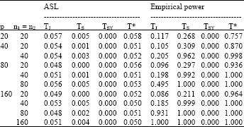
Table 1 presents the ASL and empirical powers of TJ, TS, TSY and T* when all covariance matrices in the hypothesis were under unstructured pattern (UN). The ASL of the tests TS and TSY were not close to the nominal significance level 0.05 and much lower than it for all cases considered. The test TJ generally yielded the ASL not close to 0.05 for all cases considered. Moreover, the test TJ gave the ASL around 0.060 when the sample sizes were small, n1 = n2 = 20 here and tended to increase when the sample sizes became larger for any p. For instance, when p = 80, the ASL of TJ was 0.057 (at n1 = n2 = 20) and increased to 0.061 (at n1 = n2 = 80). From this table, it is observed that the ASL of the proposed test T* were reasonably close to 0.05 and get better when p and the sample sizes increased. This is clear that the tests TJ, TS and TSY were not reasonable tests whereas the proposed test T* were. Considering the power of the test, since the competitive tests TJ, TS and TSY were not reasonable tests at this situation, then their empirical powers provided in Table 1 will be skipped. As shown from this table, the empirical powers of the proposed test T* increased to one when p and the sample sizes increased. In addition, the empirical powers of the proposed test T* increased for increasing the sample sizes when p is fixed. For instance, when p = 160, the empirical power of the proposed test T* was 0.288 (at n1 = n2 = 20) and increased to 0.944 (at n1 = n2 = 160).
| Table 1: | ASL of TJ, TS, TSY and T* under |
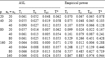 | |
| ASL: The attained significance level, U0 and U1: The matrices defined under unstructured pattern (UN), α: The nominal significance level | |
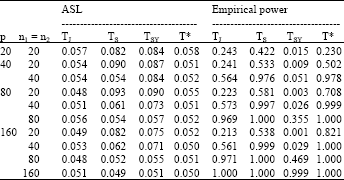
| Table 2: | ASL of TJ, TS, TSY and T* under |
 | |
| ASL: The attained significance level, C0 and C1: The matrices defined under compound symmetry pattern (CS), α: The nominal significance level | |
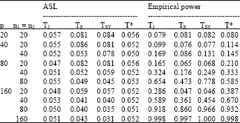
Table 2 reports the ASL and empirical powers of TJ, TS, TSY and T* when all covariance matrices in the hypothesis were set under compound symmetry pattern (CS). Both tests T* and TJ gave the satisfactory ASL which quite controlled 0.05 for all cases considered whereas those of TS and TSY were not close to 0.05. As seen in the table, the ASL of TS and TSY decreased as p and the sample sizes increased. For instance, when p = n1 = n2 = 80, the ASL of TS and TSY were 0.049 and 0.045, respectively and both decreased to 0.043 and 0.031 when p = n1 = n2 = 160, respectively. Moreover, when p is fixed, the ASL of TS and TSY were dropped when the sample sizes increased. For example, when p = 160 ASL of TS and TSY were 0.059 and 0.057 (at n1 = n2 = 20), respectively and both values decreased to 0.043 and 0.031, respectively (at n1 = n2 = 160). This indicates that the tests TS and TSY were not suitable whereas the proposed test T* and TJ test were appropriate. This table reports that the empirical powers of the proposed test T* and TJ test were quite high and rapidly tended to one. Moreover, the empirical powers of both tests were quite responsive to the increase of p and the sample sizes. Furthermore, the empirical powers of the proposed test T* were slightly higher than those of the test TJ in cases considered.
Table 3 displays the ASL and empirical powers of tests TJ, TS, TSY and T* when all covariance matrices in the hypothesis were set under heterogeneous compound symmetry pattern (CSH). We observed that the ASL of all tests under this CSH pattern were similar formats to the ASL obtained under UN pattern provided in Table 1. The ASL of the tests TJ, TS and TSY were not close to 0.05 whereas that of the proposed test T* well approximate 0.05 as p and the sample sizes increased. It can be observed that the ASL of the tests TS and TSY from this table were lower than those from Table 1 for all cases considered. This indicates that the convergences of the tests TS and TSY to the standard normal distribution were very slow and not accomplished when the common covariance matrix was under CSH and UN patterns. As displayed in this table, the empirical powers of the proposed test T* rapidly converged to one when p and the sample sizes increased.
| Table 3: | ASL of TJ, TS, TSY and T* under |
 | |
| ASL: The attained significance level, M0 and M1: The matrices defined under heterogeneous compound symmetry pattern (CSH), α: The nominal significance level | |
| Table 4: | ASL of TJ, TS, TSY and T* under |
 | |
| ASL: The attained significance level, α: The nominal significance level | |
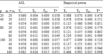
Table 4 reports the ASL of tests TJ, TS, TSY and T* under the common covariance matrix Σ = 2I (simple pattern) and their empirical powers under Σ1 = 2I and Σ2 = 1.5I. As expected, the ASL of T* and TJ were quite close to 0.05 for all cases considered while those of TS and TSY seemed to be zero for all cases considered. The empirical powers of the proposed test T* and TJ test converged to one as p and the sample sizes increased. The convergence to one of the empirical powers of the proposed test T* was extremely faster than that of TJ, especially when n1 = n2≤40 for all p. For example, when p = n1 = n2 = 20, the empirical powers of T* and TJ were 0.757 and 0.117, respectively. This indicates that, under simple pattern, T* was reasonable test and more powerful than TJ test, particularly in case of small samples.
Table 5 presents the ASL of tests TJ, TS, TSY and T* under the common covariance matrix Σ = I (simple pattern) and empirical powers under Σ1 = I and a certain matrix Σ2 = Diag (1,1,1,2, ..., 1,1,1,2).
| Table 5: | ASL of TJ, TS, TSY and T* under |
 | |
| ASL: The attained significance level, α: The nominal significance level | |
| Table 6: | ASL of TJ, TS, TSY and T* T* under |
 | |
| ASL: The attained significance level, α: The nominal significance level | |
As displayed in this table, the ASL of the proposed test T* and TJ test were similar to those from Table 4 and reasonable approximate 0.05 for all cases of p and the sample sizes. This means that changing the scalar σ2 defined in simple pattern, from σ2 = 2 became σ2 = 1, is not effected to the convergence of the asymptotic normality of the proposed test T* and TJ test. But it is greatly effected to the convergence of the asymptotic normality of TS and TSY because ASL of both tests when Σ = I were much better than those when Σ = 2I for all case considered. However, the ASL of the tests TS and TSY mainly were still not control 0.05, particularly when the sample sizes were less than or equal to 40 for any p. As expected, the empirical powers of the tests TJ and T* quickly tended to one as p and the sample sizes increased. In addition, the proposed test T* generally gave the higher power than TJ test.
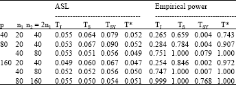
We carried out additional simulations for the case that the sample sizes were not equal (n1≠n2) choosing n2 = 2n1, of four tests TJ, TS, TSY and T* under the null hypothesis ![]() . Corresponding empirical powers of these tests were also manipulated under the alternative hypothesis
. Corresponding empirical powers of these tests were also manipulated under the alternative hypothesis ![]() and Σ2 = Diag (1,1,1,2, ..., 1,1,1,2). The results are provided in Table 6.
and Σ2 = Diag (1,1,1,2, ..., 1,1,1,2). The results are provided in Table 6.
Table 6 presents that both ASL and empirical powers of these tests were not substantially different from those given in Table 5. It appears that the tests TS and TSY still had the ASL not close to 0.05, particularly for the small sample sizes, n1 = 20 and n2 = 40 here. The proposed test statistic T* and TJ test remained appropriate even the sample sizes were not the same. The empirical powers of the proposed test T* maintained better than and converged to one faster than those of TJ test.
APPLICATION
In this section, the dataset from Notterman et al. (2001) is online at http://genomics-pubs.princeton.edu /oncology/Data/CarcinomaNormaldatasetCancerResearch.txt (last accessed: 9 October 2012). Two groups of colon tissues (adenocarcinoma and adenoma) were examined by oligonucleotide arrays. The expression levels about 6500 human genes were probed in 18 colon adenocarcinomas and 4 colon adenomas. We restricted attention to a subset of all gene expressions of 100 expression levels on 4 colon adenocarcinomas and 4 colon adenomas. Thus we had n1 = 4, n2 = 4 and p = 100. We examined whether the covariance matrices of the two groups are equal. The data presented the observed test statistic values of TJ = 0.908 and T* = -0.636. Corresponding p-values were 0.182 and 0.524 indicating the hypothesis of equality of such two covariance matrices of these data was not rejected at any reasonable significance level.
CONCLUSIONS
In this study, we proposed an alternative test statistic for testing the equality of two covariance matrices for two independent multivariate normal data with p≥ni, i = 1,2. The test statistic T* based on the consistent estimators is introduced. Its asymptotic distribution approximately follows the standard normal distribution as (p, n1, n2)→∞ even if p/ni→ci∈ (0, ∞), i = 1,2. The simulation results strongly supported the performance of the proposed test statistic T* that it accurately control size of test and not greatly affected by changing the common covariance matrix appearing in the null hypothesis. As seen in the simulation study, the proposed test statistic T* has the highest power among competitive test statistics; TJ, which is a special case of the test for testing the equality of several covariance matrices proposed by Schott (2007), TS and TSY given by Srivastava (2007) and Srivastava and Yanagihara (2010).
ACKNOWLEDGMENT
We would like to thank the Commission on Higher Education (CHE) of Thailand for financial support through a grant fund under the Strategic Scholarships Fellowships Frontier Research Networks.
APPENDIX
Most of work in this study could be viewed as an extension some results of Srivastava (2005) and Fisher et al. (2010). In order to proof Lemma 1 we have taken the following two useful lemmas (lemma A1 and A2) from Srivastava (2005).
Lemma A1: Let nS∼Wp(Σ,n) and ak = (trΣk)/p, k = 1,...,4. Then under the assumptions (A1) and (A3), unbiased and consistent estimators of a2 as (p, n)→∞ is given by ![]() .
.
Lemma A2: Let nS∼Wp(Σ,n), ![]() as defined in (2) and ak = (trΣk)/p, k = 1,...,4. Then under the assumptions (A1) and (A3):
as defined in (2) and ak = (trΣk)/p, k = 1,...,4. Then under the assumptions (A1) and (A3):
where, Φ(x) denotes the cumulative distribution function of a standard normal random variable and:
The extensions of lemmas A1 and A2 can be obtained without proofs as follow:
Lemma A3: Let ![]() and
and ![]() i = 1,2, j = 1,...,4. Then under the assumptions (A2) and (A4), unbiased and consistent estimators of a2i as (p, ni) → ∞ are given by
i = 1,2, j = 1,...,4. Then under the assumptions (A2) and (A4), unbiased and consistent estimators of a2i as (p, ni) → ∞ are given by  , i = 1,2.
Lemma A4: Let ![]() , i = 1,2, as defined in (1) and
, i = 1,2, as defined in (1) and ![]() , i = 1,2, j = 1,..., 4. Then under the assumptions (A2) and (A4):
, i = 1,2, j = 1,..., 4. Then under the assumptions (A2) and (A4):
where Φ(x) denotes the cumulative distribution function of a standard normal random variable and:
The following lemma is taken from Fisher et al. (2010). Thus it also is presented without proof.
Lemma A5: Let nS∼Wp(Σ, n) and ak = (trΣk)/p, k = 1,...16. Then under the assumptions (A1) and (A3), unbiased and consistent estimators of a4 as (p,n)→∞ is given by ![]() defined as:
defined as:
where:
 |
and
REFERENCES
- Bartlett, M.S., 1937. Properties of sufficiency and statistical tests. Proc. R. Soc. Lond. A, 160: 268-282.
CrossRefDirect Link - Dudoit, S., J. Fridlyand and T.P. Speed, 2002. Comparison of discrimination methods for the classification of tumors using gene expression data. J. Am. Statist. Assoc., 97: 77-87.
CrossRefDirect Link - Fisher, T., X. Sun and C.M. Gallagher, 2010. A new test for sphericity of the covariance matrix for high dimensional data. J. Multivariate Anal., 101: 2554-2570.
CrossRef - Gamage, J. and T. Mathew, 2008. Inference on mean sub-vectors of two multivariate normal populations with unequal covariance matrices. Stat. Probabil. Lett., 78: 420-425.
CrossRef - Huang, D., Y. Quan, M. He and B. Zhou, 2009. Comparison of linear discriminant analysis methods for the classification of cancer based on gene expression data. J. Exp. Clin. Cancer Res., Vol. 28.
CrossRef - Ibrahim, J.G., M. Chen and R.J. Gray, 2002. Baysian models for gene expression with DNA microarray data. J. Am. Statist. Assoc., 97: 88-99.
CrossRef - Notterman, D.A., U. Alon, A.J. Sierk and A.J. Levine, 2001. Transcriptional gene expression profiles of colorectal adenoma, adenocarcinoma, and normal tissue examined by oligonucleotide arrays. Cancer Res., 61: 3124-3130.
PubMed - Schott, J.R., 2007. A test for the equality of covariance matrices when the dimension is large relative to the sample size. Comput. Stat. Data Anal., 51: 6535-6542.
CrossRef - Sebastiani, P., H. Xie and M.F. Ramoni, 2006. Baysian analysis of comparative microarray experiments by model averaging. Bayesian Anal., 1: 107-732.
CrossRefDirect Link - Srivastava, M.S., 2005. Some tests concerning the covariance matrix in high dimensional data. J. Japan Statist. Soc., 35: 251-272.
Direct Link - Srivastava, M.S., 2007. Testing the equality of two covariance matrices and testing the independence of two subvectors with fewer observations than the dimension. Proceedings of the International Conference on Advances in Interdisciplinary Statistics and Combinatorics, October 12-14, 2007, Greensboro, North Carolina, USA.
- Srivastava, M.S. and H. Yanagihara, 2010. Testing the equality of several covariance matrices with fewer observations than the dimension. J. Multivariate Anal., 101: 1319-1329.
CrossRef