
Nasir Ganikhodjaev
Computational and Theoretical Sciences, IIUM, Kuantan, Malaysia
Kamola Bayram
Computational and Theoretical Sciences, IIUM, Kuantan, Malaysia
Journal of Applied Sciences
Year: 2012 | Volume: 12 | Issue: 18 | Page No.: 1978-1981


ABSTRACT
In this study, we introduce the simplest random binomial tree model. Usual binomial tree model is prescribed by pair of numbers (u, d), where u denotes the increase rate of the stock over the fixed period of time and d denotes the decrease rate, with 0<d<1<u. We call the pair (u, d) an environment of the binomial tree model. A pair (Un, Dn), where {Un} and {Dn} be the sequences of independent, identically distributed random variables with Un>1 and 0<Dn<1<Un for all n, is called a random environment and binomial tree model with random environment is called random binomial tree model. In this paper, we define and study European call option for such models.
PDF Abstract XML References Citation
Received: April 21, 2012;
Accepted: August 04, 2012;
Published: September 08, 2012
How to cite this article
Nasir Ganikhodjaev and Kamola Bayram, 2012. Random Binomial Tree Models and Options. Journal of Applied Sciences, 12: 1978-1981.
DOI: 10.3923/jas.2012.1978.1981
URL: https://scialert.net/abstract/?doi=jas.2012.1978.1981
DOI: 10.3923/jas.2012.1978.1981
URL: https://scialert.net/abstract/?doi=jas.2012.1978.1981
INTRODUCTION
A binomial tree model is extremely important, popular and useful technique for pricing an option (Cox et al., 1979; Rendleman and Bartter, 1979). In the binomial model, the market is composed of a non-risky asset B (bond), corresponding to the investment into a savings account in a bank and of a risky asset S (stock), corresponding for example, to a quoted stock in the exchange. For the sake of simplicity, we suppose that the time intervals have the same length Δt = tn-tn-1, i.e., NxΔt = T and the interest rate is constant over the period (0, T), that is rn = r/N for every interval Δ = tn-tn-1. Then the dynamics of the bond is given by:
| (1) |
So that:
It is evident that Bn converges to Bo×er. The details of compound interest are available in study of Hull (2011) and Pascucci (2011).
For the risky asset, we assume that the dynamics is stochastic: In particular, we assume that when passing from time tn-1 to time tn the stock can only increase or decrease its value with constant increase and decrease rates. Let u indicates the increase rate of the stock over the period [tn-1, tn] and d indicates the decrease rate, where 0<d<1<u.
We point out that we have:
| (2) |
Hence, a “trajectory” of the stock is vector such as (for example, in the case N = 6):
It is well-known (for example (3, 4) that the binomial tree model is arbitrage –free and complete if and only if condition:
| (3) |
The binomial tree model is a natural bridge, overture to continuous models for which it is possible to derive the Black-Scholes option pricing formula (Black and Scholes, 1973; Georgiadis, 2011; Merton, 1973).
There are two types of options: calls and puts. A call option gives the holder the right to buy the underlying asset for a certain price by a certain date. A put option gives the holder the right to sell the underlying asset by a certain date for a certain price. There are four possible positions in option markets: A long position in a call, a short position in a call, a long position in a put and a short position in a put. Taking a short position in an option is known as writing it. Options are currently traded on stocks, stock indices, foreign currencies, futures contracts and other assets. Options can be either American or European, a distinction that has nothing to do with geographical location. American options can be exercised at any time up to the expiration date, whereas European options can be exercised only on the expiration date itself. European options are generally easier to analyze.
Random binomial tree model
Random walks in a random environment: Random walks in a random environment on the integers Z was introduced and studied by Solomon (1975). Let (αn) be a sequence of independent, identically distributed random variables with 0≤αn≤1 for all n. The random walk in a random environment on the integers Z is the sequence {Xn} where X0 = 0 and inductively Xn+1 = Xn+1 (Xn-1), with probability αXn, (1-αXn). Solomon have proved that randomizing the environment in some sense slows down the random walk. Later, Menshikov and Peteritis (2001) studied random walks in a random environment on a regular, rooted, colored tree and the asymptotic behavior of the walks was classified for ergodicity or transience in terms of the geometric properties of the matrix describing the random environment.
Random binomial tree model: As mentioned above for binomial tree model during each time step the value of stock either moves up with a certain probability by u times or moves down by d times with a certain probability. Let us call the pair (u, d) environment of binomial tree model. Note that in this model pair (u, d) is the same for any moment of time.
Now we define random environment and random binomial branch model as follows. Let {Un} and {Dn} be the sequences of independent, identically distributed random variables with Un>1 and 0<Dn<Un for all n. This pair (Un, Dn) is called a random environment.
The random binomial tree model in a random environment (Un, Dn) is defined as model such that during nth moment of time the value of stock either moves up with a certain probability by Un times or moves down by Dn times with a certain probability for some realization of these random variables.
Simplest random binomial tree model: Let {Un} and {Dn} be the sequences of independent, identically distributed random variables such that the random variable Un takes only two values u1 and u2, respectively the random variable Dn takes two values d1 and d2. Thus the pair of random variables (Un, Dn) describes two possible environments (u1, d1 ) and (u2, d2).
To avoid complicated mathematical formulations let introduce and explore simplest example of random environment in binomial tree model using tossing a coin.
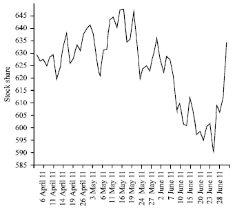 | |
| Fig. 1: | Stock shares of Rolls Royce for period from 6th April till 28th June 2011 |
Let us consider two environments (u1, d1) and (u2, d2). We will toss repeatedly a coin and if the result is “Head” we will apply first environment, in opposite case the second. That is we will choose environment randomly and we will call such model simplest random binomial tree model.
To justify necessity consideration of such models consider Fig. 1 which represents the movements of stock shares.
By examining the graph on the Fig. 1, one can see that there are two environments instead of one, namely (u1, d1) = (1.04; 0.98) and (u2, d2) = (1.02; 0.96). For this case we have two environments and they chosen randomly:
H, T, H, T, H, H, H, T, H, T, T, T, H, H, T, T, T….
One can see that this model more exactly reflects the trajectory of stock.
Theorem 1: The simplest random binomial tree model with two possible environments (u1, d1) and (u2, d2) is arbitrage-free and complete if and only if the following conditions holds:
| (4) |
where, r is the interest rate.
Proof: The proof immediately follows from similar proposition for binomial tree models with single environment. For example proposition available in study of Hull (2011) and Pascucci (2011).
Options on simplest random binomial tree models: Below we will consider simplest random binomial tree model where the randomness of environment is defined by tossing a coin (non necessarily fair) N times. Let ΩN be a sample space with outcome ω = (ω1, ω2,…, ωN), where ωi∈{H,T}, i = 1, 2, …, N, observing “Heads” or “Tails”. Note that below T is a period of time and T is Tail. Let Pr {H} = α and Pr {T} = 1-α, where 0≤α≤ 1. For any outcome ω∈ΩN we compute price of an option, i.e., construct a random variable and option price for random binomial tree model we define as expectation of corresponding random variable. In this study we consider European call option for simplest random binomial tree model. Other options are considered similarly.
Recall that the objective of the analysis is to calculate the option price at the initial node of the tree.
Options on single-period binomial tree: Firstly, we consider European call option for simplest random single-period binomial tree model. In this case N = 1, i.e., Δt = T and Ω1 = {H, T} and random environments (u1, d1) and (u2, d2) correspond to outcomes “Head” and “Tail’ respectively. Then we can compute option prices f (H) and f (T) assuming that condition (4) holds using well known formula (Cox et al., 1979; Pascucci, 2011):
| (5) |
Where:
| (6) |
Then option price f for simplest random single-period binomial tree model we define as expectation of random variable f: Ω1→R, i.e.,
| (7) |
Example 1: Let us consider simplest random binomial tree model with two environment u1= 1.1, d1 =0.9 and u2 = 1.4, d2 = 0.7. If a stock price is currently $20 and the risk-free interest rate is 12% per annum with continuous compounding, find the value of 3-months of European call option with a strike price of $21 for simplest random single-period binomial tree model.
We consider the probability of turning out of the first environment as α = 0.9 and of the second 1-α = 0.1. Such as the second environment has high u and low d, this kind of situation indicates to a crisis or too good economical state which happens seldom. So the price of an option calculated by using two environments, considering casual and extraordinary situations of market, is a more realistic one.
Using formulas from Eq. 5-7 one can compute that:
f (H) = 0.633; f (T) = 3.206
and
f = α f (H) +(1-α) f (T) = 0.890
Options on two-period binomial tree: In this case N = 2, i.e., 2xΔt = T and Ω2 = {(H, H); (H, T), (T, H); (T, T)} and random environments (u1, d1) and (u2, d2) correspond to outcomes “Head” and “Tail’ respectively.
For outcomes (H, H) and (T, T) the value if corresponding options one can compute directly using well known formula for the case of two time steps of usual binomial tree model:
| (8) |
where, fuu the value of the stock after two up movements, fud after one up and one down and fdd after two down movements. For outcome (H, T) repeated application of equation (5) gives:
| (9) |
| (10) |
Substituting from Eq. 9 and 10 into 5, we get:
| (11) |
f = α2f (H, H)+2α(1-α) f (H, T)+(1-α)2f (T, T)
and it is evident that f (H, T) = f (T, H).
Then the option price f for simplest random two-step binomial tree model is defined as expectation of random variable f: Ω2→R, i.e.,
f = α2f (H, H)+2α(1-α) f (H, T)+(1+α)2 f (T, T)
Example 2: Now let us look at the example 1 in a two steps model. Using formulas (8) and (11) one can compute that f (H, H) = 1.282; f (H, T) = f (T, H) = 3.490; f (T, T) = 3.819 and the value of our option will be f = α2 f (H, H) + 2α(1-α) f (H, T)+(1-α)2 f (T, T) = 1.705.
Options on n-period binomial tree: Suppose that a tree with N-time steps is used to value a European call option with strike price K and life T. Each step is of length T/N, i.e., NxΔt = T. For usual binomial tree model, if there have been j upward movements and N-j downward movements on the tree, the final stock price is S0 uj dN-j, where u is the proportional up movement, d is the proportional down movement and S0 is the initial stock price. Then option price f is computed as follows:
| (12) |
Now consider simplest random binomial tree model where the randomness of environment is defined by tossing a coin (non necessarily fair) N times. Let ΩN be a sample space with outcome ω = (ω1, ω2,…, ωN), where ωi∈{H,T}, i = 1, 2,…, N, observing “Heads” or “Tails”. Let Pr {H} = α and Pr{T}= 1-α, where 0≤α≤ 1. For any outcome ω∈ΩN let M (ω) be the number of tails in tossing of coin N times. If M (ω) = 0 or M (ω) = N, then one can compute option price for European call using previous formula. Now we show how to compute option price for 0<M(ω)<N. Let M (ω) = 1. Then using trivial identity (a+b)N = (a+b)N-1 (a+b), we can find option price f1 (ω) as following:
 |
Similarly for M (ω) = m, where 1≤m≤N-1, we can find option price fm(ω) as following:
 | (13) |
where, p1 and p2 one can compute using formula (6) for corresponding environments (u1, d1) and (u2, d2), respectively.
Let Am={ω∈ΩN; M (ω) = m}. It is well known that:
Now option price f for simplest random N-period binomial tree model we define as expectation of random variable f: ΩN→R, i.e.,:
| (14) |
where, m = 0, 1,…, N.
CONCLUSIONS
One way of deriving the famous Black-Scholes-Merton result for valuing a European option on a non-dividend-paying stock is by allowing the number of time steps in a binomial tree to approach infinity. This study has introduced random binomial tree model and derived formula for computing European call options for such models. Similarly one can define and study other options. To derive formula for the valuation of a European call option for random binomial tree models similar to the Black-Scholes-Merton formula for usual binomial tree models, we have to investigate:
by allowing the number of time steps to approach infinity. Since in the case of random binomial tree models we have “doubled” randomness. Also it is an interesting problem to derive the Black-Scholes-Merton differential equation with random coefficients. All these problems will be subjected in coming papers.
ACKNOWLEDGMENTS
This work was supported by the IIUM Grant EDW B 12-403-0881. The authors also acknowledges useful remarks from referee.
REFERENCES
- Cox, J.C., S.A. Ross and M. Rubinstein, 1979. Option pricing: A simplified approach. J. Financial Econ., 7: 229-263.
CrossRef - Rendleman Jr., R.J. and B.J. Bartter, 1979. Two-state option pricing. J. Finance, 24: 1093-1110.
Direct Link - Black, F. and M. Scholes, 1973. The pricing of options and corporate liabilities. J. Political Econ., 81: 637-654.
CrossRefDirect Link - Georgiadis, E., 2011. Binomial options pricing has no closed-form solution. Algorithmic Finance, 1: 1-6.
Direct Link - Merton, R.C., 1973. Theory of rational option pricing. Bell J. Econ. Manage. Sci., 4: 141-183.
CrossRef