Classification of Remote Sensing Data with Markov Random Field

The satellite observation with a resolution of ten meters provides images of earth surface. The precise spectral information allows a classification of earth objects. Due to some considerations, Markov Random Field has become a common search procedure. Attention has been focused on utilizing the spatial context in image classification; labels are to be assigned to individuals’ pixels or groups of pixels. In this approach, we relied on, among approaches to Markov Random Field to a supervised classification of satellite images. This approach is known as the Multi-Scales model. We use an energy expression according to Potts model.

INTRODUCTION

Satellite observations at resolutions of about 10 m provide images of land use. The spectral information at the terrain allows a classification of objects of land. Classification is a process aiming at the identification of the regions which constitute the image. The raw satellite image is characterized by its large amount of rich and diverse digital form.

The purpose of the satellite images analysis is to extract the maximum of information interesting for users. In our approach, we use the Random Markov Fields for a supervised satellite images classification.

Remote sensing images: The satellites provide images of the land with different space and spectral resolutions. The raw satellite images are unusable in practice. They must undergo treatments to make them exploitable (Bonn et al., 2002; Kato et al., 1993; Dubes et al., 1990).

Classification is a stage of this treatment, which aims at exploiting the maximum of information contained in these images in order to represent them in a comprehensible and interpretable form (Iftene and Mahi, 1996).

In this study, we used the satellite image of Landsat5 TM dated March 15, 1993 and representing the region of Oran in western Algeria. Data of this study area have been provided by the Spatial Researches Center Arzew-Algeria. The area concerned by our studies is marked in red in Fig. 1.

This area represents an occupation of various regions, which can be interesting due to confusions between the localization of certain classes during the use of the algorithms of traditional classification.

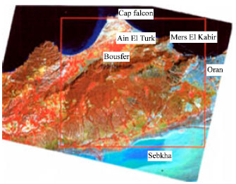Fig. 1:	Satellite image of Landsat5 TM representing the region of Oran in the west of Algeria

Classification: Generally, in a classification the data to be analysed relate to objects or individuals. The objects are characterized by a set of attributes, which constitute multidimensional observations. One associates each one of them vectors XεR_N/X=[ x₁, x₂......., x_n] where them: x₁, x₂......, x_n is N attributes used to characterize the objects to be classified among I classes, noted C_i/i = 1, 2, 3..., n.

In remote sensing the purpose of the classification of the satellite images is to assign each pixel to a particular class or topic such as sea, forest, urban, sand, scrub, cultivation of cereals, fallow land, surf, burnt land, maraichage and sebkha, based on the radiometric values of the pixels according to channels TM1, TM3 and TM4 of LANDSAT. We applied a supervised classification, because the number of classes and their characteristics are fixed at the beginning (Achab et al., 2007; Polverni and Gautret, 2001). The training must include the following stages:

•	Choice of the classes of objects in the image

•	Division of the zones of drive in group:

•	For learning to describe classes in terms of value

•	For verification or tests used for classification

•	To characterize the spectral signatures i.e., to locate them in spectral space and to evaluate their separability

•	To launch classification

•	To carry out tests of classification of the pixels occupying the zones reserved for the training

•	To carry out tests of classification of the pixels occupying the zones reserved for the checking

Our attention is related to the random fields of Markov like a classification tool, because these last years the MRF became increasingly popular, especially in the image processing.

In this study we used the algorithm of recuit simulated on the image modelled by the random fields of Markov with the model of energy of Potts.

Markovian model: Classification within the framework of the image processing consists in assigning, according to a criterion, the pixels of the image to the class to which they belong.

Among these probabilistic methods, the random fields of Markov (Markov Random Field-MRF), were increasingly popular, in the last few years, in the image processing (Smits and Dellepiane, 1996; Bouman and Shapiro, 1994).

Several reasons made adopt the fields of Markov like mode of research. One of them it is the increasing attention related to the role of the space context in the classification of the images, in which label with pixels or groups of pixels are assigned (Kato et al., 1992; Lorette et al., 1998).

Definition of a neighborhood and a click:

•	S = {s1,s2,s3,.......,sN } a set of points. Gs: the neighbors oh the point s

•	G = {Gs/s∈S} is a neighborhood system of S if : s ∉ Gs

•	C ⊆ S is called a clique if any pair of sites in C are neighbors

•	We denote by D the set of cliques, deg (D) =Max C∈D |C|

Gibbs distribution and MRF: X = {X_s/s∈S} is a family of random variables such that: ∀ s∈S: X_s∈Λ avec Λ = {0, 1, 2, ...., L-1} represents the state space any.

Ω = {w = (w_s1, w_s2, w_s3, ........., w_sN): w_si ∈Λ ; 1≤ i ≤ N} the set of all possible configurations.

The distribution of Gibbs relating to the system of vicinity is the measurement of probability π in Ω such as:

(1)

where, Z is a constant of standardization or a function of partition:

(2)

Where,

T	:	Constant called temperature
U	:	Function of energy of the form:

(3)

Where:

V C

:

Function called potential, it is defined in and it depends only of

The relation between the distribution of Gibbs and the MRF' S is summarized in the theorem of Hammersley-clifford which is announced as follows:

X is random fields of markov respecting the system of vicinity G if and only if π (w) = P(X = w) is a distribution of Gibbs.

Markovian model of classification of image: X is a MRF relating to the system of vicinity G with a function of potential energy U₂ and one V_C

Such as:

(4)

And

(5)

To find classification optimal, one uses the rule of Bayes the classification which maximizes the distribution with posterior P(X=w/F) (Rignot and Chellappa, 1993):

P(X=w/F) =P (F/X=w) P(X=w) / P (F)

As P (F) is independent of W, then P (F) is constant, the MAP estimator is to give by:

(6)

(7)

To find a solution optimal of the Eq. 6, we used the algorithm of simulated recruit.

Algorithm ICM (iterated conditional mode): Proposed by Besag this algorithm converges quickly with a MAP optimal estimator. It is given by:

•	To choose the initial configuration W0 k = 0 and E> the 0 threshold

•

k = k+1 and to go to 2) until|U (w^K)-U (w^k-1)|<E

Within the framework of this study, we used approach ICM. This last uses the model multi-scale.

Markov model multi-scale: Supposing that S = {s1 s 2...., s NR} a grid (W*H), such as:

S≡Γ = {(i, j) 1<=I<=W and 1<=J<=H}

where, W = w^N and H = h^m

That is to say G a system of vicinity on these sites and X a MRF on G with the function of energy U and the potential energies {V_C}_C ε_D (Kato et al., 1993; Kato, 1994; Bouman and Liu, 1991; Derin and Elliott, 1987). The following process generates a model multi-scale:

•

•	For all 1< = I < = M (M = Inf(n, m)); S is divided into blocks of size (W1 * HI). These blocks form a scale B1 = {b1I, b2I, b3I....., bNorI} with: NI = N/(w*h)I

The classes assigned with the sites of a block are the same ones; the classes common to the block B_K¹ are noted by the forced generates a space of configuration Ω₁ which is a subset of original space .

For each 0≤i≤M: Ω_i ⊆ ⊆i-1 ⊆......⊆₀≡one consider the system of vicinity on a scale I It is clear that b_K¹ and b_L¹ are close if and only if, there are two neighbors and Then there are the same ones click that in D.

Click Them are defined in the following way: that is to say d = Deg (D), for 1≤J≤D: the whole of the blocks C_J¹ container J sites on the scale, I is one clicks of order J if there is one clicks CεD ( is with being said one clicks on the finest scale) such as:

The whole of click on scale I is noted by D¹ (D⁰D). The whole of all click them which satisfy a and b for C¹_J given is noted by:

One shares the original unit D in several following disjoined sets:

For each 1≤J≤D; that is to say A^I_J the whole of click CεD for which:

There is one click C^I_J which satisfies a and b by considering the definition of D and A^I_J one obtains:

(8)

By using this decomposition, the function of energy U can be written like continuation:

(9)

where, the potential ones of one click C^I_J of order J on scale I, we obtain on the scale B¹ the potential following ones:

(10)

To simplify the model, one associates a unique site to every block. These sites have the common label of the corresponding block and they form a coarse S¹ that is isomorphs to the ladder corresponding Bⁱ (Fig. 2).

The space of configurations on the coarse scales is isomorphous with Ω₁. Isomorphism Φ¹ of S¹ to B¹ is only one projection of the field on the coarse labels on the grid the finest

Fig. 2:	Isomorphism Φi between Bi and Si

where, Φ¹ keeps the same system of vicinity on S¹ as out of B¹ Click on S¹ inherit the potentials click defined on B¹. These grids form a pyramid, where level I contains the grid S¹ The energy of level I (i = 0..., M) is given by:

(11)

I = 0, ...., M

Where:

(12)

The algorithm multi-scales will solve the problem of minimization by using a strategy of descent in the pyramid. Each lower level is initialized by the result obtained in the preceding layer. The algorithm is given by:

•	Either and let us divide S in blocks of the size W1xH1 (1≤ I≤M). To assign a single site with each block. These sites form a coarse grate.

•	Calculate the potentials on the coarse grids by using the Eq. 6.

•	Either i = M. Find the global minimum of U1 in Eq. 7

•	Initialize the layer (i-1) by the projection of

•	If i = 1 then stop, otherwise return to Step 4. With I = i-1

The advantages of this algorithm are clear. Each gives an estimator to least good of the final result and the higher levels are simpler to solve because the space of configuration has less elements.

Application of the model multi-scale: It is supposed that the size of a block is n X n, i.e., w=h=n. Thus we obtain:

(13)

Where:

And

The values of pⁱ, q¹ depend on the size of the blocks and the system of vicinity. p¹ is the number of click pertaining to the same block on the scale Bⁱ.

q¹ is the number of clicks which are between two neighbour blocks on the scale Bⁱ.

In considering the blocks of size n x n and a system of vicinity of order 1, we obtain:

p¹ = 2n¹ (nⁱ-1)

q¹ = nⁱ

•	β: is the hyper parameter which controls the homogeneity of the areas

Algorithm of the model multi-scales: One needs two entries: the image observed and the parameters (average) and (Standard deviation) of each class. This amounts to:

•	To establish the pyramids and to calculate the parameters μi and σi on the coarse grids

•	To calculate the energies

•	To minimize the energies in the pyramid with a downward strategy

•	To take the final etiquette on the finest level as being final result of classification

Application of the MRF to the satellite image: By considering the zone of study, the result of the applications based on the Markovian approaches always depend on the samples of the departure and the value of the Beta parameter (Rabahi and Ismail, 2003; Kaddar and Fizazi, 2009). Consider the following example (Fig. 3).

In our case, we have not only applied the algorithm Multi-scale to the satellite image, but we made a variation of parameters. To do this, we chose two steps:

Fig. 3:	Classified images of each level

•	To fix the samples and to vary the parameter Beta

•	To fix the parameter Beta and to vary the samples

First step: Initially, we based ourselves on the variation of the parameter β, which is used to control the homogeneity of the areas. With each scale, we have a new value of the energy, which depends on to the parameter β. In our experiment, we varied parameter β from 0.001 to 3.0.

RESULTS

During our experiments, we noticed that the parameter β has an influence on the classification. In order to better analysis and to interpret the results, we gathered all the results obtained, for each class and various values of the parameter β.

For instance we consider β = 0.001 and classifies it Sea, one has that 12.11 % of the Sea topic in the totality of the classified image. We have expressed as a percentage to gather the preceding results by curves indicating the variations each topic according to β (Fig. 4).

According to the results obtained, we notice that there are apparent confusions on the level of following areas: Sea and surf, Sebkhat and scrub, Sebkhat and fallow land. That is noted by the means of the curves so above and classified images obtained below.

It is noticed that starting from the value β = 0.50, the Sea and the Surf are stabilized. This stability is due to the homogeneity of the sea zones and surf. In other words, the pixels of each class are gathered in the same mass.

One also notes a very great confusion between the topics: fallow land, Sebkhat and Scrub. This is due to an overlapping between the classes. For stage this degradation, one increases β until reaching value 3.0.

This is highlighted starting from the preceding graph where it is noted that there are no more confusions between the topics.

To illustrate the confusions obtained in our results and to show the influence of the parameter β on confusions, we schematised them by the Fig. 5-7.

This approach allows us to say that the parameter β can solve the problem of confusion between the various classes and that it can be regarded as parameter of improvement of classification since the images obtained correspond to the field reality.

Second step: It consists to fix β and vary the samples in order to make a classification. For that, we based ourselves on the values of the parameter β of the preceding experiments having given an image close to the reality, in other words, in which the areas are distinct. A better illustration of this step, is shown in Fig. 8 and 9 which present the results of the classification, as well as the rate of classification Tc for two choices of samples.

Fig. 4:	Curve of variation expressed as a percentage of each topic according to parameter β

Fig. 5:	Results of classification according to parameter for area fallow land

Fig. 6:	Results of classification according to parameter β for area scrub

Fig. 7:	Results of classification according to parameter β for area surf

Fig. 8:	Result of classification for the first sample Tc = 90.26%

Fig. 9:	Result of classification for the second sample Tc = 95.45%

DISCUSSION

To validate the results obtained in this article, we have compared them with those obtained in (Achab et al., 2007). The researchers of this study used the MRF model single-grid to classify the same regions shown in Fig. 1. The results show that the classification rate in the case of MRF-multi-scale Tc = 95.45 is significantly higher than the MRF model single-grid Tc = 58.68 where they are a lot of confusions between classes. There is even a total lack of the burnt class, while in the MRF-multi-scale all classes are present and the result of the classification matches the reality.

We compared our results with those obtained using K-means (Iarkani and Amel, 2008). The parameter to be determined in the K-means is the value of k that represents the number of classes (in our case k is equal to 12). The best recognition rate obtained in their work is Tc = 83.01%, but with a persisting confusions between classes sebkhat and urban, sand and land.

Our approach has improved the classification rates and the results obtained correspond to the reality.

CONCLUSIONS

For the selected method Models Multi-scales and for the steps considered, we noticed that the results obtained depend highly on the choice of training samples.

In our first step, which consists in fixing the sample and varying the parameter, we noted that confusion persists on the Sebkhat level, scrub and fallow land. That is highlighted by Fig. 5.

For stage this degradation, one can add other data such as the slope, altitude, etc As regards the second step, which consists to fix Beta and vary the sample, the results obtained show a clear improvement of classification compared to the first step. That is well to illustrate by Fig. 6 and 7.

The results obtained starting from the experiments showed, that by making a good choice of the sample and β parameter we can minimize confusions and improve classification of the satellite images by the random fields of Markov, approaches Multi-scales.

The development of fast and robust algorithms for processing and analysis of this type of data is therefore of great importance. It has been demonstrated recently that a Markov-random-field (MRF) model, based on the statistical properties of imaging, provides an ideal framework processing remote sensing data The proposed approach improves classification accuracy when applied to the segmentation of multispectral remotely sensed images with ground truth data.

REFERENCES

- Achab, K., H. Fizazi and B. Sidaoui, 2007. Design of a hybrid system for neuro-markovian classification of satellite images of the area West of Oran. National Conference on Engineering of Electronic CNIE�2007, Faculty of Electrical Engineering, University of Sciences and Technology of Oran Algeria. June 24-27.
- Bouman, C.A. and B. Liu, 1991. Multiple resolution segmentation of textured images. IEEE Trans. Pattern Anal. Mach. Intell., 13: 99-113.
Direct Link - Bouman, C.A. and M. Shapiro, 1994. A multiscale random field model for bayesian image segmentation. IEEE Trans. Image Process., 3: 162-177.
Direct Link - Derin, H. and H. Elliott, 1987. Modeling and segmentation of noisy and textured images using Gibbs random fields. IEEE Trans. Pattern Anal. Mach. Intell., 9: 39-55.
Direct Link - Smits, P.C. and S.G. Dellepiane, 1996. Data fusion in a Markov random-field-based image segmentation approach. Proc. Image Signal Process. Remote Sens. III, 2955: 85-95.
CrossRefDirect Link - Rignot, E. and R. Chellappa, 1993. Maximum a posteriori classification of multifrequency, multilook, synthetic aperture radar intensity data. J. Opt. Soc. Am. A, 10: 573-582.
CrossRefDirect Link