ABSTRACT
Extended Kalman filter is the first algorithm applied to nonlinear state estimation problem and following its limits, other methods based on sampling were developed. We can consider two categories of particle filters: filters which apply a deterministic sampling as the famous unscented Kalman filter and those whose principle is the random sampling as the Particle filter. Furthermore, other approaches that take these two forms of sampling were proposed as Sigma Point Particle filter. The major difficulty of these methods is the computation time which is related to the complexity of sampling. Particle Filter is one among the methods that has attracted particular interest recently; however, PF suffers the problem of degeneration of particles that occurs after re-sampling. We propose to improve PF by the bioinspired algorithm Particle Swarm Optimization as these 2 models have several common. The hybrid method developed in this study is called PFPSO. The PFPSO reduces significantly the degeneracy of the particles; empirical results obtained by applying PFPSO to the problem of estimating the trajectory of a mobile robot illustrate robustness and computational efficiency of our approach.
PDF Abstract XML References Citation
How to cite this article
DOI: 10.3923/jas.2010.494.499
URL: https://scialert.net/abstract/?doi=jas.2010.494.499
INTRODUCTION
Being nonlinear and non Gaussian most of the time, the general form of a discrete-time nonlinear dynamic system is modelled in Eq. 1 and 2, where: Xk is the unobserved state at step k. Let P(X0) be its initial distribution, its evolution is related to a Markovian process having P(Xk|Xk-1) as a density function. The noted observations Zk are independent and related to Xk, they are generated according to the density function P(Zk|Xk).
![]() | (1) |
![]() | (2) |
Where:
uk | = | A known exogenous input |
vk | = | A process noise with the distribution P(vk) |
P(nk) | = | The distribution of the observation noise |
f | = | The transition function |
h | = | The observation function |
P(Xk|Xk-1) | = | Defined by f and P(vk), h and P(nk) define the probability P(Zk|Xk), the estimating state is obtained by a recursive process |
Nonlinear systems are often sullied with noises related at the same time on the process of state and the collected observations. Kalman filter (Kalman, 1960) is applied to Gaussian linear systems with discrete or continuous states; its success was in short following the state models evolution, being nonlinear non-Gaussian in majority.
PF is a method based on sampling has the advantage of being applied to any type of system, however it has some form of degeneracy due to the increase in the variance of samples (Doucet et al., 2001).
To remedy this problem, other researches has been conducted and resulted in algorithms such as Sigma Point Particle Filter (SPPF) also known as Unscented Particle Filter (UPF) (Van der Merwe et al., 2000), GMSPF (Gaussian Mixture Sum Particle Filter) (Van der Merwe et al., 2003) and so on. These approaches have helped to correct the particles, thus, the problem of computing time was inevitable. The second part of this study is devoted to the main methods for filtering nonlinear systems, given next Particle Swarm Optimization (PSO) (Kennedy and Eberhart, 1995; Clerc, 2004) will be briefly defined following a comparison of PF and PSO. Both of PF and PSO use random sampling at initialization stage and the correction of the particles for searching the best solution, Table 1 shows similarities between these two approaches.
Table 1: | Comparison of PF and PSO: Comparison |
![]() | |
The PF is a Markovian process, so each particle at step k remembers only its previous state k-1, in fact, the particles in PSO are designed to save on memory all previous states.
FILTERING NONLINEAR SYSTEMS
Unscented Kalman Filter (UKF): Extended Kalman filter EKF (Kalman, 1960) was the first filter applied to nonlinear dynamic systems, supposing state process distribution, observation and all noises Gaussian. The principle of EKF is founded on linearization of functions f and h by adopting a first order Taylor development, then, after obtained a linear system, Kalman filter will be applied. This approach does not take into account the uncertainty of states around the mean; for this reason EKF diverge in most time.
Julier and Uhlmann (1997) and Wan and Van der Merwe (2001) introduced a new approach called Unscented Kalman filter or Sigma Point Kalman filter, assuming that the fundamental task in filtering and estimation is to calculate statistics of the random variable representing state. They propose to approximate mean and covariance through nonlinear transformation called unscented transformation. Let x be a random variable with mean and covariance Px, a set of points can be generated from the rows or the colons of matrix
where l is the size of the vector x. These points have 0 mean and covariance Px. By adding
to each point, we obtain a set of 2l symmetric points which have the same statistics, we have then 2l+l Sigma vectors forming a new matrix, weights Wi are associated to these vectors here k ε R,
is the ith row or colon related to the square root of (l+k)Px (Eq. 3). To calculate the statistics of the observation variable Zi, Sigma points are propagated through the nonlinear equation Zi = h(Xi), i = 0,
.,2l:
![]() | (3) |
UKF filtering is applied to the augmented variable obtained by the concatenation of the original state vector and noises vectors. We observe that particles are generated in a deterministic way because they are extracted from the covariance matrix.
Particle Filter (PF): PF, also known as sequential Monte Carlo method (Doucet et al., 2001) is a sophisticated estimation technique based on simulation; its usually used to estimate Bayesian models. The PF expresses a prior distribution by using a set of a weighted particles. Providing the prior density P(X0), itll be easy to construct the posterior probability P(Zk|Xk). Assuming that the importance density function is π(Xk|Zk) and all particles (i = 1..N) are drawn from this distribution, that is to say:
![]() | (4) |
Based on PF,
![]() | (5) |
Where:
![]() | (6) |
Therefore, as the samples were drawn from an importance density, the weights in Eq. 6 are defined to be:
![]() | (7) |
Normalized weights of particles are:
![]() | (8) |
When we obtain a measurement at time k, the particles and their weights can be computed recursively by using these formulas. After several iterations, only one particle will probably have a larger weight, the others will be equivalent to zero. This degeneracy can be expressed by the variance of the importance weights, this is remedied in the so called re-sampling stage: eliminate samples with low importance weight and multiply those having high weights.
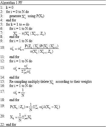
Although, the re-sampling step reduces the effects of the degeneracy problem, it introduces other inconvenience. The particles that have high weights are statistically selected many times, this leads to a loss of diversity among the particles as the resultant sample will contain many repeated points, this problem, is known as sample impoverishment, complete description of PF is shown in Fig. 1.
![]() | |
Fig. 1: | Algorithm PF |
Sigma-point Particle Filter (SPPF): PF has the advantage of being applied to nonlinear and non-Gaussian systems. The major problem of PF is the degeneration; an idea suggested (Van der Merwe et al., 2000) was to move the particles towards a space with high probability. Instead of generating them in an indeterminist way, a Gaussian distribution will be used. Van der Merwe et al. (2000) supposed that since, the Unscented transformation makes it possible to capture a random variable statistics as well as possible former, the alternative is to use UKF for all particles which offers a better approximation of state. This new filter named SPPF (Sigma-Point Particle Filter) is viewed as hybridization between PF and UKF.
Particle swarm optimization (PSO): PSO have been suggested by Kennedy and Eberhart (1995). They estimate that finding a source of food is similar to finding a solution in a common field of research. The PSO is initialized randomly with a population of stochastic particles; each particle is characterized by a position and a speed. Positions and speeds are adjusted as the particle moves. At each iteration, all particles keep track of their coordinates which are associated with the best solution their have achieved so far (pbest) and the coordinates which are associated with the best solution achieved by any particle in the neighborhood (gbest).
Each particle updates its position and its speed according to the following system Eq. 9-10, where, v is the speed of the particle, X is the current particle (solution), rand is a random number between 0 and 1, c1 and c2 are constants representing social confidence coefficients as follow:
c1 | = | How much particle trusts its experience |
c2 | = | How much particle trusts its neighbors |
![]() | (9) |
![]() | (10) |
Several variants and parameters were suggested for this algorithm and in particular the values of c1 and c2; we will consider the values of c1 and c2 in our tests as follows:
c1 = c2 = 2, this assignment is the most used to ensure equity between the local experience and the neighborhood one of the particle. Some versions of PSO were proposed and adapted to different problems, we can find an overview of this approach (Clerc, 2004).
PFPSO
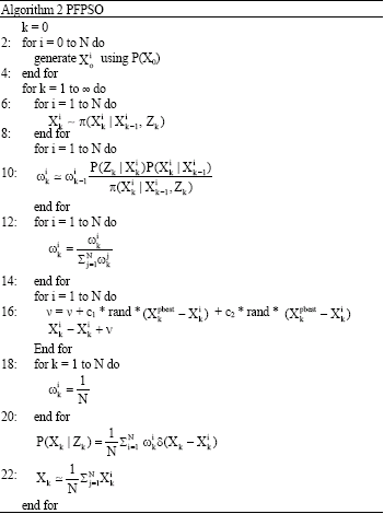
In this approach called PFPSO, we propose to use PSO to reduce the degeneracy of PF: let consider the best particle at step k over its previous steps having the higher weight which represents the best hypothesis and
the best particle in the neighborhood of the particle. Unlike Zhang et al. (2008), we suggest replacing re-sampling step of PF by one iteration of PSO equations, thus, for each particle are applied the tow equations below:
![]() | (11) |
![]() | (12) |
This will allow us to retain more diversity in the samples.
The process is Markovian, in fact, the system does not keep in memory all previous states, so, will be defined only in relation to Xk and Xk-1. The problem does not arise for gbest that will be assessed against all the particles in step k.
![]() | |
Fig. 2: | Algorithm 2 PFPS |
Resulting samples will be used for the calculation of the new solution Xk as:
![]() |
where, N represents the number PF particles.
The main advantage of our approach is that it ensures convergence towards the best solution; the variance is not likely to increase rapidly with the number of iterations as in PF because no particles will be eliminated regardless of their weight and the risk of degeneracy will be reduced, it will not be entirely avoided but will occurs more later, the cost in computing time will not be affected, this is due to the simplicity of the 2 equations of PSO. The PFPSO is more defined in Fig. 2.
RESULTS AND DISCUSSION
Zhang et al. (2008) have recently proposed a new approach called PSO-PF, they address the same problem of degeneracy of PF where they propose to fix the particles after re-sampling step, they use the 2 equations of PSO, considering a number of PSO iterations for each iteration of PF.
![]() | |
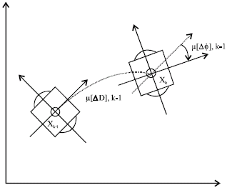
Fig. 3: | Displacement of the robot since step k-1 at |
The purpose of their algorithm is to avoid the degeneracy occurred by eliminating/multiplying particles with low weight. This method has yielded a better result compared to the traditional PF, the major drawback is that this has caused a slowdown in the computing time that was predictable.
The aim of this study is not to measure our new approach with PSO-PF but to support the idea that the 2 PF and PSO algorithms have similarities and are most effective when they are hybridized.
In application, we should estimate the trajectory of a mobile robot equipped by a sensor materialized by a GPS, this GPS permit to obtain measures where the robot will be able to localize its position. All numerical results presented in this paper were done by simulation.
It should be considered that the state and the observation models are multimodal, the robot moves using a command, its situation is defined by the co-ordinates x, y and the orientation φ. State process is attacked by a noise formulated as vk~N(0, Qk) where, Let Xk be the state vector at step k, we have:
![]() |
movement will be modelled compared to a relative displacement: distance covered ΔD and rotation Δφ as illustrated in Fig. 3. Let μk be the vector representing this displacement, we have:
![]() |
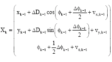
The state model is representing as :
![]() | (13) |
The observation system will have to measure the state of the robot by means of sensors. Let,Zk be the observation variable, this vector will represent the same co-ordinates exactly as those of the state vector; the difference is that these co-ordinates are obtained by the measurement system installed.
![]() | (14) |
The assumptions on the observation noise are the same ones as for the state noise; this process is random and Gaussian, its modelled by nk where, nk ~N(O, Rk) and . We applied PF, SPPF and PFPSO to estimate the trajectory of a robot which will carry out a rectangular trajectory, this trajectory is discretized to 205 states.
For all these methods, we have considered the case of 200 particles, the choice of the optimal number should take another study and we do not approach it in this article, this is why we choose to fix N to the value of 200. We tested both these algorithms 100 times and results represent the average of the overall error and the average of computed time obtained over 205 steps. The error estimated (e) is computed as the Euclidian distance ek between the real state and the estimated one xk where:
![]() |
From the results shown in Table 2, it is evident that SPPF is the approach that gave the best estimate of the trajectory with a global error around 7. However, SPPF has taken a considerable time (more than 2 h), this represents a real handicap for the purpose of filtering methods where the goal is to find the best estimate on a real-time status.
![]() | |
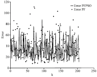
Fig. 4: | The estimation error by PF and PFPS |
![]() | |
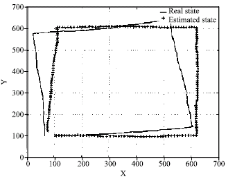
Fig. 5: | PF estimation |
![]() | |
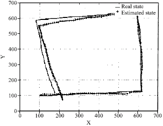
Fig. 6: | PFPSO estimation |
An improvement was noted as we can deduce in Fig. 4 which shows estimating errors of PF and PFPSO over 205 steps; Fig. 5 shows one run of PF and Fig. 6 Shows one run of PFPSO, we can see the deviation of the robot from the real trajectory in PF, therefore, we can observe a superposition of the real trajectory of the robot and that estimated in the case of PFPSO until a certain point where degeneration appears, the degeneracy is not avoided completely but was significantly reduced and occurs more later.
Table 2: | Error and computing time |
![]() | |
This improvement depends on particles, instead of being eliminated they will be adjusted, i.e., their positions will be shifted towards the best solution. We can not guarantee the elimination of degeneracy because it depends on the weight of sample: if its strongly weak compared to the best weight, the improvement will be then relative, also, PSO has the inconvenience of achieving the optimum local. The computing time is still unchanged; the reason is that all particles will be adjusted in both cases PF and PFPSO. Error and CPU time are shown in Table 2.
CONCLUSION
In conclusion we can resume that our method is more efficient than the traditional PF, the Particle Filter presents a certain degeneracy but it reacts better if itll be combined with another approach like PSO as found by Zhang et al. (2008) and in our work. Both of these two improving algorithms dont eliminate absolutely the problem; the principal reason is the problem of reaching the optimum local. We have considered in this study the basic form of PSO, in future, it would be interesting to explore deeper PF and PSO and take into account their parameters; in particular the optimal number N of particles for PF and the constants c1 and c2 for PSO, also, we suggest testing different topologies of PSO in our proposed algorithm, this should probably give another interesting discussion.
ACKNOWLEDGMENTS
This acknowledgments are intended to University of Science and Technology of Oran and in particular to Laboratory of Simulations and Modelling of Industrial Systems which has placed at our disposal the necessary material and a suitable environment for carrying out this work.
REFERENCES
- Kalman, R.E., 1960. A new approach to linear filtering and prediction problems. Trans. ASME. J. Basic Eng., 82: 35-45.
Direct Link - Kennedy, J. and R. Eberhart, 1995. Particle swarm optimization. Proc. IEEE Int. Conf. Neural Networks, 4: 1942-1948.
CrossRefDirect Link - Julier, S.J. and J.K. Uhlmann, 1997. A new extension of the kalman filter to nonlinear systems. Proceedings of the 11th International Symposium on Aerospace/Defense Sensing, Simulation and Controls, April 21-24, 1997, Orlando, FL., USA., pp: 1-12.
Direct Link - Van der Merwe, R. and E. Wan, 2003. Gaussian mixture sigma-point particle filters for sequential probabilistic inference in dynamic state-space models. Proceedings of the Acoustics Speech and Signal, (ASS'03), China, pp: 701-704.
CrossRef - Zhang, G., Y. Cheng, F. Yang and Q. Pan, 2008. Particle filter based on PSO. Proceedings of the International Conference on Intelligent Computation Technology and Automation, Intelligent Computation Technology and Automation, Oct. 20-22, ICICTA, pp: 121-124.
CrossRefDirect Link