
R. Sokouti
Research Center of Agricultural and Natural Resources of West Azarbaijan, P.O. Box 365, Uromieh, Islamic Republic of Iran
M.H. Mahdian
Soil Conservation and Watershed Management Institute, Iran
Journal of Applied Sciences
Year: 2009 | Volume: 9 | Issue: 3 | Page No.: 588-592


ABSTRACT
The present research was conducted to analyze spatial changes in soil salinity distribution as an aspect of soil degradation and to compare the efficacy of different Geostatistical methods in its estimation and the preparation of maps of the spatial distribution of soil salinity. To estimate soil salinity of non-sampled areas, the methods of Kriging, Co-Kriging and Weighted Moving Average were applied in Geographical Information System (GIS) medium. To evaluate the efficacy of the methods, the cross-evaluation approach with two statistical parameters of mean bias error and mean absolute error was taken in practice. Results indicated the high precise of Kriging method with regression coefficient of 0.98 for the estimation of salinity rates in the areas, for where no data were available before. Estimation error for this method was 1.31 and biass was -0.34 dS m-1 which indicates high accuracy of Kriging method to estimate topsoil salinity and its precise.
PDF Abstract XML References Citation
How to cite this article
R. Sokouti and M.H. Mahdian, 2009. Comparative Efficacy of Some Geostatistical Methods for the Estimation
of Spatial Variability of Topsoil Salinity. Journal of Applied Sciences, 9: 588-592.
DOI: 10.3923/jas.2009.588.592
URL: https://scialert.net/abstract/?doi=jas.2009.588.592
DOI: 10.3923/jas.2009.588.592
URL: https://scialert.net/abstract/?doi=jas.2009.588.592
INTRODUCTION
Soil salinity is the most important constraint to agricultural sustainability, but accurate information on its variation and its impact on agricultural regions are difficult to obtain (Lobella et al., 2007). Monitoring soil salinity requires knowledge of its magnitude and its spatial and temporal variability. The method used depends on the data availability and the aim of the study. The joint use of temporal stability and temporal mean shift and spatial shift tests could result in a drastically reduced sampling effort (Douaika et al., 2007). So, spatial changes of various soil traits such as its salinity may be one of the main error sources in the estimation of the non-measured data. Corwin et al. (1992) have implied to the necessity of the application of Geostatistical methods in the compensation for the defects encountered with the above-mentioned methods. Accordingly, geostatistical methods like non-parametrical statistical estimators such as weighed moving average and or parametrical Geostatistical methods such as Kriging and Co-Kriging attract attentions. Because of taking in account of spatial correlation of data, Geostatistical methods are of high importance in the studies related to the distribution of earth data (Goovaerts, 1999).
The results obtained by Alaeddin et al. (2007) suggested that sampling cost can be reduced and estimation can be significantly improved using cokriging. Walter and McBratney (2001) used Kriging method in order to predict soil surface salinity in his analytical studies on the spatial distribution of soil salinity. Triantafilis et al. (2001) resulted to more accuracy of Co-Kriging method than ordinary Kriging or other univariate predictors.
Mohammadi (1998) concluded that the calculated variograms were mainly in accordance with spherical and exponential models. Corwin et al. (1992) applied GIS and successfully estimated salinity of the lands under irrigation. Lesch et al. (1995) mapped soil salinity distribution using calibrated spectrometric data. Mohammadi (2000) compared the efficacy of different Geostatistical methods including Co-Kriging, Kriging and linear regression methods and found that the Geostatistical estimators were relatively superior to linear relations and introduced Kriging method as the superior method for the estimation of soil spatial data.
Geostatistics offers a collection of deterministic and statistical tools aimed at understanding and modeling spatial variability (Goovaerts, 1999; Triantafilis et al., 2001).Therefore the present research was conducted to analyze spatial changes in soil salinity distribution as an aspect of soil degradation and to compare the efficacy of different Geostatistical methods in its estimation and the preparation of maps of the positional distribution of soil salinity.
MATERIALS AND METHODS
Area identification: The investigation was performed in Southern part of Orumieh plain in West Azerbaijan province, Iran. Geographically, this area is longitudinally located 45°05’ 00" E and 45°20’ 00" E and between 37°15’ 00" N and 37°35’ 00" N. Figure 1 shows the location of the region in the country and province and shows the position of the profiles used in the plain. Based on the relatively detailed pedological studies made in Water and Soil Research Institute (2000), the regional soils are classified in the class Inceptisols and belong to one of two main subgroups, typical Calcixerepts and typical Haploxerepts. The distance between the profiles in the studied region varied between 1300 and 4700 m. Extensive soil salinity is observed around the Uromieh Lake and in parallel to its coasts.
Research framework: Geostatistical methods including Kriging, Weighed Moving Average and Co-Kriging methods (Metternicht and Zinck, 2003) were used in GIS medium and GS+ and ARCVIEW8 software (Goovaerts, 1999) were applied to investigate the spatial changes and the estimation of superficial soil salinity. The general equation for these methods is as follow:
Where:
| Z* (xi) | = | The estimated amount |
| Z (xi) | = | The observed amount around the assumed point |
| (xi) | = | The position of the observed points |
| λ i | = | The amount of weights of the observed points |
| N | = | No. of the measurement points |
To evaluate interpolation methods, the cross validation technique and two MAE and MBE statistical parameters were used. MAE is an indicator of errors in the results and MBE indicates the biass of the results obtained through the applied method. When MAE and MBE are 0.00 or near to naught, the applied method simulates the fact well. However, as far as its amount is farer than 0.00, it implies to less precise and more biass. How the parameters MAE and MBE are calculated, has been indicated as follow:
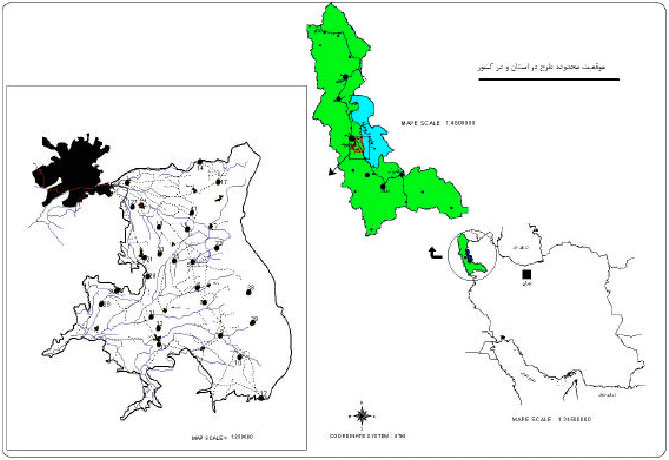 | |
| Fig. 1: | Location of the study area and soil profiles |
 |
Where:
| Rs | = | The estimated amount |
| Ro | = | The measured amount |
| N | = | No. of the data |
Spatial distribution of surface soil salinity was mapped after the selection of the appropriate interpolation model. This map was compared with the photos taken with the satellite through multi-spectral combination method (Metternicht and Zinck, 2003) and salinity borderlines and the trend of regional salinity variations were reviewed and tested.
RESULTS
Shapiro-Wilk test conducted to see if the data were of normal distribution, indicated that the data related to soil salinity were normal and of a coefficient less than 0.05 and their skew ness coefficient was less than 1 (df = 26; calculated test coefficient = 0.035 and skewness coefficient = 0.568).
To follow Kriging and Co-Kriging methods, calculation of semivariogram is a pre-requirement. The resulted model for Kriging method has been shown in Fig. 2. The performed studies indicated that the Gaussian Model is an appropriate model for this semi- variogram. The effect radiance of this semivariogram is equal to 8000 m, nugget effect equals 1.4 and its sill is equal to 41.28 m2. The correlation coefficient for the fitted model has been calculated as 0.98.
Also, there was a significant correlation between soil salinity and lime content (R = 0.74); therefore, lime content was used as a co variable with the Co-Kriging method. The empirical semi-variogram model obtained through this method indicated that Gaussian model was a suitable model for semi-variogram. The effect radiance of this semi-variogram is equal to 10000 m, its nugget effect is 0.26 and its sill equals to 4.53 m2 with a correlation coefficient of 0.58.
As Fig. 3-5 shows the results from the cross-validation test of selected geo-statistical methods, the Kriging method-based fitted line obtained from the estimated data is of more fitness with the measured data. The rates of preciseness and biass with Kriging, Co-Kriging and weighted moving average have been shown in the Table 1.
 | |
| Fig. 2: | Empirical semi-variogram model of soil salinity using the Kriging method, Gaussian model (Co = 1.40000, Co+C = 41.28000, Ao = 2900.00, R2 = 0.980, RSS = 11.5) |
 | |
| Fig. 3: | The cross validation of soil salinity estimation following the Co-Kriging method, Regression co-efficient = 1.614 (SE = 0.871, R2 = 0.125, y-intercept = -1.44, SE prediction = 6.555) |
 | |
| Fig. 4: | The cross validation of soil salinity estimation following the weighted moving average method, Regression co-efficient = 1.236 (SE = 0.209, R2 = 0.594, y-intercept = -0.70 SE prediction = 4.468) |
 | |
| Fig. 5: | The cross validation of soil salinity estimation following the Kriging method, Regression co-efficient = 0.941 (SE = 0.304, R2 = 0.285, y-intercept = 0.35, SE prediction = 5.924) |
 | |
| Fig. 6: | Comparing the regions classified as saline land with their position in the false color TM satellite image |
| Table 1: | The error and biass values of the selected geostatistical methods used in the estimation of soil salinity levels |
 | |
Based on the information presented in Table 1, it is confirmed that Kriging method with an error rate of 1.31 dS m-1 is more preciseness for the estimation of soil salinity. While Co-Kriging method is less biass compared to the Kriging method (-0.09 dS m-1), this difference is only at the rate of 0.20 dS m-1. Therefore, considering the preciseness and biass rates and the Kriging method would be the most superior method.
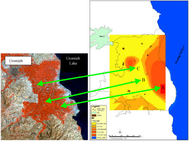
Thus, because of its more preciseness, Kriging method was chosen as the appropriate model for the spatial estimation of soil salinity and the salinity levels were estimated for various regional points and their regional distribution maps were prepared in GIS medium (Fig. 6). The comparison of the points classified as saline lands shown in Fig. 6 are in good accordance with the satellite image. Based on this, the regional trend of salinity variation is in a way that saline lands have been extended paralleled to Orumieh coastal lines (Region A). The breadth of these areas depends on the land topography and the level of lake brine penetration inside coastal lands. In better words, the rate of brine penetration is of more extension in the lands of mild slopes (Region B). The lands located in the central and west southern and classified as the relatively saline lands are under the effects of physiographic situation and are considered as low lands (Region C).
DISCUSSION
The results obtained with the present investigation, namely the selection and recommendation of Kriging method are in agreement with those published by Mohammadi (1998), Walter and McBratney (2001) and apposite with Triantafilis et al. (2001) results. This indicate the spatial regularity of soil salinity data but it differs in different regions. The fitted model in this research was Gaussian model for semi-variogram; however, in a research by Mohammadi (1998) exponential and spherical models have been resulted. Also, using the satellite-based calibrated spectral and numerical data, Lesch et al. (1995) and Mohammadi (2000) have made a TM digital data, however, the correctness of the prepared maps have not been tested and in no case of the reviewed literature on the comparison of different geo-statistical methods, statistical methods have been applied in comparisons.
REFERENCES
- Lobella, D.B., J.I. Ortiz-Monasteriob, F.C. Gurrolac and L. Valenzuelad, 2007. Identification of saline soils with multiyear remote sensing of crop yields. Soil Sci. Soc. Am. J. 71: 777-783.
CrossRef - Douaika, A., M.V. Meirvenneb and T. Tóthc, 2007. Statistical methods for evaluating soil salinity spatial and temporal variability. Soil Sci. Soc. Am. J., 71: 1629-1635.
CrossRef - Metternicht, G.I. and J.A. Zinck, 2003. Remote sensing of soil salinity: Potentials and constraints. Remote Sens. Environ., 85: 1-20.
CrossRefDirect Link - Goovaerts, P., 1999. Geostatistics in soil science: state-of-the-art and perspectives Geoderma, 89: 1-45.
CrossRefDirect Link - Triantafilis, J., A.I. Huckel and I.O.A. Odeh, 2001. Comparison of statistical prediction methods for estimating fieldscale clay content using different combinations of ancillary variables. Soil Sci., 166: 415-427.
Direct Link - Alaeddin, A.T., B.E. Abbassi, R.A. Taany and G.A. Saffarini, 2007. Spatial variability of topsoil salinity in the lower reaches of Zerka River, Central Jordan Valley. J. Food Agric. Environ., 3: 368-373.
Direct Link - Walter, C. and B. McBratney, 2001. Spatial prediction of topsoil salinity in the Chelif Valley, Algeria, using local ordinary Kriging with local variograms versus whole-area variogram. Aust. J. Soil Res., 39: 259-272.
Direct Link