
A. Valizadeh
Department of Civil Engineering, Tarbiat Modares University, Tehran, Iran
M. Shafieefar
Department of Civil Engineering, Tarbiat Modares University, Tehran, Iran
J.J. Monaghan
School of Mathematical Sciences, Monash University, Clayton, Australia
S.A.A. Salehi Neyshaboori
Department of Civil Engineering, Tarbiat Modares University, Tehran, Iran
Journal of Applied Sciences
Year: 2008 | Volume: 8 | Issue: 21 | Page No.: 3817-3826


ABSTRACT
The basic equations governing the free surface flow of a fluid are considered and approximated by using a semi-compressible Smoothed Particle Hydrodynamics (SPH) method which is a grid-less Lagrangian approach. It is found that the standard SPH method, which has been successfully applied to simulate the transient free surface flows, could be used for simulation of multiphase flows with high density ratios, by doing a correction on mass of interface particles. The SPH modeling is shown to provide a promising tool to predict the two liquid characteristics of free surface flows. To show the validity of the present method numerical examples on bubble rising in a heavier fluid and luck-exchange flow are considered and a good agreement is observed.
PDF Abstract XML References Citation
How to cite this article
A. Valizadeh, M. Shafieefar, J.J. Monaghan and S.A.A. Salehi Neyshaboori, 2008. Modeling Two-Phase Flows Using SPH Method. Journal of Applied Sciences, 8: 3817-3826.
DOI: 10.3923/jas.2008.3817.3826
URL: https://scialert.net/abstract/?doi=jas.2008.3817.3826
DOI: 10.3923/jas.2008.3817.3826
URL: https://scialert.net/abstract/?doi=jas.2008.3817.3826
INTRODUCTION
The Smoothed Particle Hydrodynamics (SPH) method is a powerful particle approach which was originally developed for the study of astrophysics (Monaghan and Gingold, 1983; Monaghan, 1988) and later employed to study the wave overtopping over coastal structures (Dalrymple and Rogers, 2006; Gomez-Gesteira and Dalrymple, 2004). In the simulations of incompressible flows using the SPH model, the incompressibility is achieved by employing an equation of state and the fluid is assumed to be slightly compressible, which is called the weakly compressible SPH method. In SPH method, materials are approximated by particles that are free to move around rather than by fixed grids or meshes. The particles are basically moving interpolation points that carry with them physical properties, such as the mass, velocity, viscosity, density of the fluid and any other properties that are relevant. The inter-particle forces are calculated by smoothing the information from nearby particles in a way that ensures that the resultant particle motion is consistent with the motion of a corresponding real fluid, as determined by the Navier-Stokes equations.
Despite its fully Lagrangian property, when the standard formulation of SPH is applied to multi-phase flows only small density differences are permitted between the considered phases because it is implicitly assumed that the density gradient is much smaller than that of the smoothing kernel (Monaghan, 1994; Monaghan and Kocharayan, 1995; Monaghan et al., 1999). As a remedy, Ritchie and Thomas (2001) suggest a summation of the particle-averaged pressure, not density, to handle large density gradients. However, their method does not satisfy mass conservation. Colagrossi and Landrini (2003) modified the approximation form of spatial derivatives to diminish the effects of large density difference across the interface. Nevertheless, since the density summation is replaced by a non-conservative density evolution equation mass conservation is not satisfied either. Although the conservation errors are decreased somewhat by a special density re-initialization approach, they may accumulate and affect the flow behavior considerably in long time computations. Hu and Adams (2006) employed a particle smoothing function in which neighboring particles only contribute to the specific volume but not to the density. The resulting algorithm resolves a density discontinuity at a phase interface naturally and satisfies mass conservation since a density summation equation was employed, this method was suffering from clumping and clustering, so Hu and Adams (2007) developed an incompressible SPH model which solves the Poisson equation for pressure by a projection formulation. This model is a good model for two phase flows. The scope of this study is finding a quick and simple way for correction the standard semi-compressible SPH model, for high density difference multiphase flows. The essential step is that by changing the mass of particles which have interaction with particles from a different phase, the undesirable force between two particles is controlled, this simple idea improves the results very well and comparison model`s results with previous numerical, analytical and experimental results supports this claim.
In the present study, first the general concepts of the standard SPH modeling for incompressible flows are given. On this ground, the present SPH-implementation is introduced and described in details and derived graphs for mass coefficient in a case that light fluid is surrounded by a heavy fluid (e.g., bubble rising in water) are presented. Using these graphs the lock-exchange flow for different fluids is simulated and compared with experimental works and other numerical models.
MATERIALS AND METHODS
SPH is a particle based method for modeling coupled fluid flows, solid structure deformation and heat transfer. The particles represent blobs of discretised fluid or solids that move around in response to the fluid or solid stresses produced by the interaction with other particles. Importantly, SPH does not use any fixed grids or meshes to track the fluid and calculate the fluid velocities. Formally, SPH is a Lagrangian continuum method for solving systems of partial differential equations. The fluid (or solid) is discretised and the properties of each of these fluid/solid elements are attributed to their centers, which are then interpreted as a particle. SPH uses an interpolation kernel to smooth the values of any information held by the particles to give smooth continuous interpolated fields.
Governing equations: The almost incompressible medium water is not made totally incompressible but more compressible in SPH. The full mass conservation equation has to be used:
(1a) |
(1b) |
(1c) |
The Eq. 1a-c give a time derivative of the density, velocity and the position of fluid particles. ρ, u, v, x, t represent the density, velocity, viscosity, position and time, respectively and fd is a body force such as gravity. With a relation between the pressure and the density it is no longer necessary to solve the implicit Poisson equation for the pressure.
Numerical model: In SPH, the fluid field is represented as a collection of N neighbor particles, interacting each other through evolution equations of the general form:
(2a) |
 | (2b) |
(2c) |
where, ρi, ui, Pi, mi, xi are the density, velocity, pressure, mass and position of particle i, fi is a body force, IIij is the viscous term and Wij = W(rij, h) is the smoothing function. rij = ri−rj is the position vector from particle j to particle i and h is the smoothing length. By neglecting the atmospheric pressure, the state equation between pressure and density is as follow (Batchelor, 1974):
(3) |
where, ρi and ρi are the reference pressure and density of fluid, γ = 7, P0 = c2ρ0/γ and c is the used speed of sound and instead of using the real sound speed which needs using a very small time step for the stability reasons, an artificial sound speed of c ≈ 10 μmax is used in SPH. With this value for speed of sound, the maximum relative density differences are small in order of ~ 1% (Monaghan, 1994). Now the calculation time stays reasonable and water is only slightly compressible in SPH. In multi-phase flows P0, ρ0, c and γ may be different for each phase. The quartic spline kernel which is used here is in this form
 | (4) |
where, q = rij/hij, rij is the absolute distance between particles i and j and. The spatial derivative of kernel function for two dimension problems is calculated as:
(5) |
The choice of the smoothing length h is determining the number of interactions for each particle. When h is too small, there are not enough particles nearby to interact with, giving a low accuracy. When h is too big, local properties are smeared out too much, this gives a low accuracy again and the calculation becomes slow. Here an adaptive kernel function is used by defining a variable smooth length, using the following equation (Monaghan, 2005).
(6) |
where, d is the number of dimensions. According to this formula the smooth length is increasing by decreasing in density and vice-versa. So, in places such as interface between two phases or near the boundaries, kernel function adopts itself to the conditions. With a smoothing length around 1.4 times the initial particle spacing, Δp, the circle of influence has a radius of 3.5 and 2.8 Δp for quartic and cubic spline functions, respectively. With this smoothing length every particle has 36 and 20 neighbors in two dimensions for mentioned functions, respectively. That is a good optimum for both accuracy and calculation speed.
II ij is the viscous term and is defined as an artificial viscous stress term. Different methods for defining this term have been produced by scientists (Monaghan, 1994; Cleary, 1998; Gomez-Gesteira and Dalrymple, 2004). One of the prevalent definitions which is used in this study is (Monaghan, 2005).
(7a) |
(7b) |
 | (7c) |
![]() is the average density.
is the average density. ![]() , this is the velocity difference between two particles.
, this is the velocity difference between two particles. ![]() is the constant for defining the viscosity difference between two particles and α is chosen normally between limits 1 > α > 0. β is a coefficient which in all simulations is equal to 2. This artificial viscosity introduces both shear and bulk viscosity, but with neglectable changes in the density it is almost entirely shear viscosity. This approach to model viscosity guarantees that momentum is transferred from the particle with the highest velocity to the particle with lowest velocity.
is the constant for defining the viscosity difference between two particles and α is chosen normally between limits 1 > α > 0. β is a coefficient which in all simulations is equal to 2. This artificial viscosity introduces both shear and bulk viscosity, but with neglectable changes in the density it is almost entirely shear viscosity. This approach to model viscosity guarantees that momentum is transferred from the particle with the highest velocity to the particle with lowest velocity.
Colagrosi and Landrini (2003) showed that the averaging of the densities helps ensure that the free surfaces are smooth and physically acceptable and Dalrymple and Rogers (2006) performed this filtering every 40 time steps by reinitializing the density of each particle according to:
 | (8) |
In this study, the reinitialisation of density is done every 40 time steps for each phase separately, it prevents of density deviations and keeps the density of particles near to reference density.
The XSPH correction for movement of particle is included according to Eq. 9, it means an average between the particle`s velocity and the average field velocity from all neighbor particles is used for moving a particle in Eq. 2c. This smoothing on velocity prevents particles penetration. Also for consistency reasons, the smoothed velocity has to be used in continuity equation. It should be noted that the new smoothed velocity is used just in Eq. 2a and c and in the momentum equation the non-smoothed velocity is used (Monaghan, 1989).
 | (9) |
where, ε is a constant (0 < ε < 1). With ε =1 the particles are moved with the field velocity, with ε = 0 the particles are moved with their own velocity, normally ε = 0.5.
Time integration: By using the SPH approximation, three differential equations should be integrated in time:
(10a) |
(10b) |
(10c) |
These differential equations are integrated in time by using the predictor-corrector time integration which predicts the velocity, density and particle position at the intermediate time steps, as follows:
Predictor step:
(11a) |
(11b) |
(11c) |
where, An, An+1/2 and An+1 denote the value of variable A at the beginning, intermediate and at the end of (n+1)th time step, respectively.
Corrector step:
(12a) |
(12b) |
(12c) |
With these predictors the time integration is second order accurate. The time step, δt, is calculated according to the Courant condition modified for the existence of viscosity:
(13) |
δto is the initial time step, h is the smoothing length, σ is a coefficient between zero and one, normally σ = 0.5 and vσ is defined in Eq. 7b.
Boundaries: Boundaries in SPH can be modeled by virtual particles that characterize the system limits. Basically, three different types of particles can be distinguished:
| (a) | Boundary particles with repulsive forces: The closed boundary is modeled with a single row of boundary particles with mass, fixed density equal to fluid particles density and no pressure. Their positions are fixed or external imposed during the calculation (Fig. 1a). A repulsive boundary force is used to stop approaching fluid particles in analogy with the forces among molecules (Monaghan, 1994, 2005). |
| (b) | Quasi fluid boundary particles: One or more rows of fixed fluid particles are placed at the boundary. No estimates of boundary forces or directions are needed; the boundary particles just like fluid particles verify equations of continuity and state, except that their position is fixed or externally imposed in time. They build up pressure just like normal fluid particles; this is how they prevent particle penetration. Fluid particles near the boundary have interaction with a double staggered row of quasi-fluid particles. When a slip boundary is needed these quasi fluid particles are used in the calculation of the viscous stress terms, for a free-slip boundary they are not used (Crespo et al., 2007). |
  | |
| Fig. 1: | Modeling of closed boundaries in SPH method, (a) boundary particles with repulsive force and (b) ghost particles, dark particles are fluid and gray particles are ghost particles |
| (c) | Ghost particles: For every particle within a distance shorter than the kernel support radius (e.g., 2 hi for cubic spline function) from the boundary, a virtual (ghost) particle is mirrored outside the boundary every time step (Randles and Libersky, 1996). Both particles have same mass, density and pressure, but velocities normal to boundary are opposite. The velocities parallel to boundary can be the same in sleep boundaries and opposite for non-slip ones (Fig. 1b). |
In this research the closed boundaries are simulated by ghost particles; the main advantage of this method is that boundary is compatible with different phases and it can adopt itself with fluid particles. Because we are working with particles with different characteristics, especially with different mass and densities, the boundary is adaptive with particles. By using fixed particles for closed boundary, either quasi-fluid particles or repulsive force particles, there will be difficult to simulate an adaptive boundary which can be compatible with different phases. Also, using particles with repulsive forces impose an undesirable kinetic energy in system which needs some initial time steps for damping this energy. For problems which start with an instability such as bubble rising or dam breaking, initial damping of the kinetic energy is difficult but by using ghost particles the amount of initial kinetic energy is small and there is no need to initial damping.
In this study, the bottom and wall friction are defined by selecting the velocity of ghost particles in direction parallel to boundary in this form
(14) |
where, ug and uf are the parallel to boundary velocity components of ghost and fluid particles, respectively and Cv is a coefficient which defines the amount of friction and slip or non-slip boundary (−1≤Cv≤1), in Fig. 1b this coefficient is equal to 0.3.
Correction in standard SPH: The standard SPH which is used for simulating two liquids with different density ratios, works well for density ratios greater (ρl/ρd) (than 0.1, but for smaller density ratios it suffers from different problems. At smaller density ratios, because particles attain large velocities in opposite directions on the two sides of the interface, the instability occurs sooner and the solution rapidly deteriorates. We understood that the main source of increasing velocities in the interface is the mass differences between two particles which are belong to two separate fluids; this mass difference in momentum equation causes the increase of the rate of velocity changes. So, we concentrated on changing the mass of particles which have interaction with particles from other fluid artificially. Two coefficients have been defined as cmd and cml which are the coefficient of mass of dense fluid and light fluid, respectively. When a particle from denser fluid interacts with a particle from lighter fluid, the masses of these particles are changed as follows:
(15) |
In order to finding a regular method for defining these coefficients, several tests with different particle sizes for different density ratios have been done for evolution of rising a circular bubble through the initially still heavier fluid. The brief of these simulations is that, as density ratio goes to one or particle size goes to zero, the value of coefficients cmd and cml goes to one.
MODEL VERIFICATIONS
The bubble rising in a heavier liquid: We found that numerical stability of a two-phase flow model with SPH in a case that lighter fluid is surrounded by a denser fluid is more difficult than a case which denser fluid is surrounded by lighter fluid. In this case a circular bubble of fluid A is free to rise through the initially still fluid B. we suppose that surrounding liquid is water (ρw = 1000 kg m-3) and the simulations are done for bubbles with different characteristics. According to the experimental and analytical results (Batchelor, 1974; Liu and Zheng, 2006; Kwaguch et al., 2006), if the volume of a bubble in water increases beyond 0.0006 cc, the bubble becomes oblate, owing to the variation of pressure in the water over the surface of the bubble and it is also observed to rise in an oscillatory manner. Further increasing in the bubble volume is accompanied by a progressive flattening of the rear face of the bubble and for volume above 5 cc, for which surface tension is negligible, the bubble is shaped like an umbrella. The rear face is rather unsteady and the edge of the slice is jagged and irregular, but by contrast the whole of the front appears to be steady, smooth and closely spherical or in two dimension circular (Fig. 2). Here we consider the general shape of bubble and the speed U with which the bubble rises through the water. According to analytical solution of Batchelor (1974) and comparison with experimental results (Davis and Taylor, 1950) for a wide range of bubble sizes and different liquids the following formula has been produced for two-dimensional bubbles:
(16) |
 | |
| Fig. 2: | Photograph of air bubble in nitrobenzene; R = 3 cm, U = 0.37 m sec-1 (Simplified from Davis and Taylor, 1950) |
 | |
| Fig. 3: | Comparison of SPH results (—) for bubble rise (rear face of bubble) with analytic formula (−) (Batchelor, 1974), ρl/ρd = 0.001, cmd = 1.0, cml = 2.5, dp = 0.04 and R = 0.28 m |
where, R is the radius of curvature of the bubble surface and g is the gravity acceleration. ρd and ρl are, respectively the density of surrounding liquid and bubble. In the case of bubble rising, if cmd be selected less than one, particles of bubble will spread among water particles and this is not desirable, also for high density ratio using mass coefficients equal to one result in deterioration of model. So for balance the forces from near interface particles, the mass of lighter particles should be increased by selecting cml greater than one. The position of rear face of air bubble, ρ = 1 kg m-3 with radius equal to 0.28 m in a tank of water, ρw = 1000 kg m-3 is compared with analytical formula (Eq. 16). There is a time lag between two results, because in SPH model, an initial interaction between particles, causes a bit decreasing in volume of bubble, but by shifting the graph of SPH to left a good agreement is considered (Fig. 3). In this simulation the artificial viscosity coefficients of air and water are 0.001 and 0.01, respectively. For finding proper cml for bubbles with different densities in water and for different particle sizes, the shape and speed of rising bubble are considered. The final values for cml are shown in Fig. 4. In all simulations which have been done for finding the proper cml, an agreement similar to Fig. 3) should be achieved and the shape of rising bubble should be similar to Fig. 2 and 5.
By rise of bubble, the circle or changes to a mushroom shape and then the tail of bubble is separated by vortex current and finally there is an umbrella shape bubble with a flat rear face (Fig. 2, 5). By increasing the density ratio and decreasing the particle size and increasing the resolution of model the amount of cml is going to one. In all simulations the value of cmd is equal to one, just for density ratios larger than 0.5, for reaching at exact speed of bubble rising, there is need to increasing the mass of surrounding particles by choosing cmd greater than one, in these cases cml should be chosen greater than one for keeping the shape of bubble in correct form.
 | |
| Fig. 4: | The values for cml against density ratio of two fluids. Different graphs show different particle sizes; -◊-, -□- and -Δ- represent particle size of 0.02, 0.04 and 0.05, respectively |
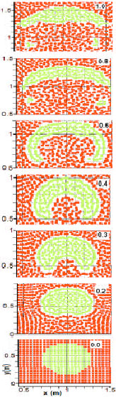 | |
| Fig. 5: | Air bubble rising in water, The frames show the position and shape of bubble from bottom to top at times 0.0, 0.2, 0.3, 0.4, 0.6, 0.8 and 1.0 sec. The conditions are similar to Fig. 3 |
For this case study one fluid was surrounded by another one, completely, but in a lot of practical problems, there is a changeable interface between two phases. In these cases it is possible to choose special amounts for cml and cmd by an engineering judgment according to results of this section; here we want to model lock-exchange between two fluids with high density ratios using the mentioned method.
High density ratio lock-exchange flow: Lock-exchange flow is a good test for direct numerical simulations of flows of large density difference fluids. When a horizontal channel is divided into two parts by a vertical splitter plate and each chamber is filled with a fluid of different density, an intruding, gravity-driven flow occurs when the splitter removed. It consists in the spread of a dense current of the heavier fluid under the lighter fluid and a lighter fluid current above the heavier fluid, as is shown in Fig. 6. This referred to as lock-exchange flow. In the experiments by Gröbelbauer et al. (1993), gases with a density ratio of up to 21.6 were released in an unevenly divided horizontal channel of half-height H = 0.15 m, as shown in Fig. 6. The lock gate could be placed at a distance 20 H from the right or left wall and 10 H from the other one. The passage time of either the light or dense front was measured at fixed positions on the horizontal walls of the larger chamber and the Froude number of each front for the various gas pairs was calculated.
Table 1 shows the pairs of used gases and the range of conducted numerical simulations.
 | |
| Fig. 6: | Lock-exchange flow, experimental setup used by Gröbelbauer et al. (1993) H = 0.15 m |
The dynamic viscosity μ of these gases lies between 12.57x10⁻⁶ Pa sec (freon 22), 18.64x10⁻⁶ Pa sec (helium) and 21x10-6 Pa sec (argon), while the kinematic viscosity (v) ranges from 3.43x10⁻⁶ m2 sec-1 (freon 22) to 1.10x10⁻⁴ m2 sec-1 (helium). Thus, it is natural to keep the dynamic viscosity constant in the attempt to reproduce these experiments by numerical simulation. This might be different for liquids. At the interface between the dense and light fluids, shear-layer instabilities develop which give rise to Kelvin-Helmholtz billows. The smoke visualization by Gröbelbauer et al. (1993), indicates some instability on the interface especially close to the dense front when the density ratio is large. As long as this instability remains two dimensional, its essential features are accurately captured by the direct numerical simulations. In order to validate the numerical simulations presented in this study, the conditions of the experiments Gröbelbauer et al. (1993) were reproduced as closely as possible. The parameters of four of these experiments reproduced by numerical simulation are shown in Table 1. The characteristic Reynolds number of these flows was calculated with the viscosity μ and density of the lighter gas, Re = ρlUh/μl. By using the SPH method the kinematic viscosity is calculated from this formula (Monaghan, 2005).
(17) |
The coefficients for dense and light particles, cmd and cml are also shown in Table 1). An adaptive kernel function which its smoothing length varies according to the changing of density is used here for increasing automatic and unconstrained resolution in intrusion fronts, which have steep density and velocity gradients. It is assumed that for all amounts of β, the three-dimensional effects are negligible, so it is possible to use the two-dimensional numerical model for decreasing computational costs.
In Fig. 7 the numerical results of our SPH model are compared with the experimental results of Gröbelbauer et al. (1993) and with numerical results of Étienne et al. (2005).
For the light front the agreement between the arrivals of the simulated and the experimental fronts is as well as the results of Étienne et al. (2005).
| Table 1: | Values of the density parameter ρ* and Reynolds numbers in the experiments of Gröbelbauer et al. (1993) and in the numerical simulations presented here |
 | |
| vl = μl/ ρl, Re = ρlUh/μl, | |
  | |
| Fig. 7: | Comparison of the numerical and experimental results, (a) light front and (b) dense front. For lock-exchange, in all cases, Exp: Experimental results of Gröbelbauer et al. (1993), FE: Finite Element model of Étienne et al. (2005), SPH: Current SPH model, ρd = 1000 kg m-3 and α = ( ρd– ρl)/ ρd |
  | |
| Fig. 8: | Comparison of the numerical and experimental results for Froude numbers, (a) Light front and (b) dense front, ρd= 1000 kg m-3 and α = ( ρd– ρl)/ ρd |
For the dense front, a nearly constant shift in time between the calculated and measured front arrivals is observed (Fig. 7b) similar to Étienne et al. (2005) numerical results. Possible explanations for this time shift according to reasoning of Étienne et al. (2005) are either a large numerical inconsistency in time around t = 0 or a time lag in the measurements. Thus, we are left to suppose that there is either a uniform time lag in the measured arrival time of the front, which may be due to a detection problem, or that the time shift is due to the opening of the gate.
In Fig. 8a and b, the experimental and numerical Froude numbers ![]() of light and dense fronts for different density ratios are compared. Since the Froude number only accounts for the established velocity of the front, the shift in front arrival between numerical and experimental results has no effect.
of light and dense fronts for different density ratios are compared. Since the Froude number only accounts for the established velocity of the front, the shift in front arrival between numerical and experimental results has no effect.
It is shown from Fig. 8a that, for the light front, the SPH model is in close agreement with the experiments of Gröbelbauer et al. (1993) and also with numerical results of Étienne et al. (2005), numerical and experimental results concerning Frl deviate from the straight line![]() . Figure 8b shows that for the dense front, the SPH model as well as the model of Étienne et al. (2005), for Reynolds numbers corresponding to the experiments of Gröbelbauer et al. (1993), fit closely the experiments. The data points can be closely fitted by a power law of the form
. Figure 8b shows that for the dense front, the SPH model as well as the model of Étienne et al. (2005), for Reynolds numbers corresponding to the experiments of Gröbelbauer et al. (1993), fit closely the experiments. The data points can be closely fitted by a power law of the form ![]() .
.
In Fig. 9 the shape of lock-exchange flow and nondimensional vorticity for β = 0.11, at two stages in the flow development is shown. The vorticity of each particle is defined as (Monaghan, 1992):
(18) |
The general shape of vorticity is approximately similar but is not in excellent agreement. This may be improved by doing some correction on vorticity formula in SPH and by increasing the resolution of SPH model.
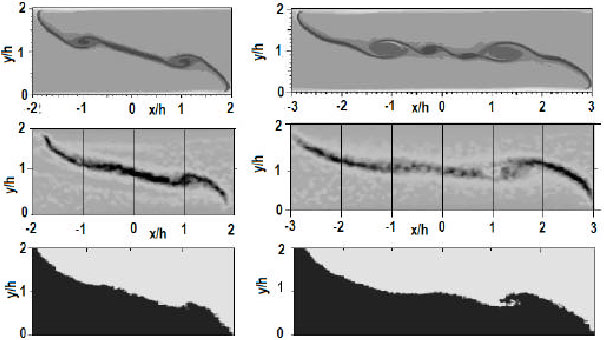 | |
| Fig. 9: | Comparison of vorticity at the interface of two fluids, top to bottom, vorticity from Étienne et al. (2005), vorticity from SPH and the density profile, respectively |
CONCLUSION
A multi-phase free surface flow implementation of Smoothed-Particle Hydrodynamics (SPH) is presented and a new correction on standard SPH is provided. In this model without defining the interface between two phases or using complicated correction for standard SPH method and just by changing the mass of particles which have interaction with particles from other phases according to derived graphs from bobble rising in a heavier fluid and an engineering judgment, it is possible to model the violent two-phase free surface fluids with density ratios ( ρd/ ρl) up to 1000. Numerical examples are investigated and compared with analytic solutions, previous results and experiments. The results suggest that this method can be faithfully applied to multi-phase flows. Since its construction is based on the standard SPH method the involved corrections are simple to implement and suitable for straightforward extension to three dimensions.
ACKNOWLEDGMENT
The authors gratefully acknowledge Iranian Water Resources Management Co. support through grant ENV1-84120.
REFERENCES
- Batchelor, G.K., 1974. An Introduction to Fluid Mechanics. 4th Edn., Cambridge University Press, Cambridge, UK., ISBN: 0521663962 pp: 635.
Direct Link - Cleary, P.W., 1998. Modelling confined multi-material heat and mass flows using SPH. Applied Math. Model., 22: 981-993.
CrossRefDirect Link - Colagrossi, A. and M. Landrini, 2003. Numerical simulation of interfacial flows by smoothed particle hydrodynamics. J. Comput. Phys., 191: 448-475.
CrossRefDirect Link - Crespo, A.J.C., M. Gomez-Gesteria and R.A. Dalrymple, 2007. Dynamic boundary particles in SPH. 2nd International Workshop on SPHERIC-Smoothed Particle Hydrodynamics, May 23-25, 2007, Madrid, Spain, pp: 152-155.
Direct Link - Dalrymple, R.A. and B.D. Rogers, 2006. Numerical modeling of water waves with the SPH method. Coastal Eng., 53: 141-147.
CrossRefDirect Link - Davies, R.M. and G. Taylor, 1950. The mechanics of large bubbles rising through extended liquids and through liquids in tubes. Proc. R. Soc. London Series A, Math. Phys. Sci., 200: 375-390.
Direct Link - Étienne, J., E.J. Hopfinger and P. Saramito, 2005. Numerical simulations of high density ratio lock-exchange flows. Phys. Fluids, 17: 036601-036601-12.
CrossRefDirect Link - Gomez-Gesteira, M. and R.A. Dalrymple, 2004. Using a 3D SPH method for wave impact on a tall structure. J. Waterway Port Coast. Ocean Eng., 130: 63-69.
CrossRefDirect Link - Gröbelbauer, H.P., T.K. Fanneløp and R.E. Britter, 1993. The propagation of intrusion fronts of high density ratios. J. Fluid Mech., 250: 669-687.
Direct Link - Hu, X.Y. and N.A. Adams, 2006. A multi-phase SPH method for macroscopic and mesoscopic flows. J. Comput. Phys., 213: 844-861.
CrossRefDirect Link - Hu, X.Y. and N.A. Adams, 2007. An incompressible multi-phase SPH method. J. Comput. Phys., 227: 264-278.
CrossRef - Liu, Z. and Y. Zheng, 2006. PIV study of bubble rising behavior. Powder Technol., 168: 10-20.
CrossRefDirect Link - Monaghan, J.J. and A. Kocharyan, 1995. SPH simulation of multi-phase flow. Comput. Phys. Commun., 87: 225-235.
CrossRefDirect Link - Monaghan, J.J. and R.A. Gingold, 1983. Shock simulation by the particle method SPH. J. Comput. Phys., 52: 374-389.
CrossRefDirect Link - Monaghan, J.J., 1989. On the problem of penetration in particle methods. J. Comp. Phys., 82: 1-15.
CrossRefDirect Link - Monaghan, J.J., 1992. Smoothed particle hydrodynamics. Ann. Rev. Astronom. Astrophys., 30: 543-574.
CrossRefDirect Link - Monaghan, J.J., 1994. Simulating free surface flows with SPH. J. Comput. Phys., 110: 399-406.
CrossRefDirect Link - Monaghan, J.J., 2005. Smoothed particle hydrodynamics. Rep. Prog. Phys., 68: 1703-1759.
CrossRefDirect Link - Monaghan, J.J., R.A.F. Cas, A.M. Kos and M. Hallworth, 1999. Gravity currents descending a ramp in a stratified tank. J. Fluid Mech., 379: 39-69.
Direct Link - Randles, P.W. and L.D. Libersky, 1996. Smoothed Particle Hydrodynamics-some recent improvements and applications. Comput. Methods Applied Mech. Eng., 139: 375-408.
CrossRefDirect Link - Ritchie, B.W. and P.A. Thomas, 2001. Multiphase smoothed-particle hydrodynamics. Mon. Not. R. Astron. Soc., 323: 743-758.
CrossRefDirect Link