
Yadan Mao
Institute of Geophysics and Geomatics, China University of Geosciences, Wuhan, 430074, Hubei, China
Journal of Applied Sciences
Year: 2005 | Volume: 5 | Issue: 2 | Page No.: 207-214


ABSTRACT
The relation between the particle displacement and the strain field is introduced. Then, stress field is related to the particle velocity by the equation of motion. Based on that, Hooke`s law provides a way to link stress and strain fields through elastic parameters characterizing the medium. Finally, Christoffel equation is obtained and T is presented by Thomsen. Its plane wave solutions for solid of transverse isotropy of vertical symmetry axis (TIV). Since the transverse isotropy or hexagonal symmetry is the simplest anisotropy case of widespread geophysical applicability, the author then describes transverse isotropy (TIV) by five elastic parameters, using the main notations introduced by Thomsen in 1986. For ray tracing purposes, the difference between the phase and group velocities is clarified in order to numerically derive the change in ray velocity due to anisotropy.
PDF Abstract XML References Citation
How to cite this article
Yadan Mao, 2005. Understanding the Anisotropy. Journal of Applied Sciences, 5: 207-214.
DOI: 10.3923/jas.2005.207.214
URL: https://scialert.net/abstract/?doi=jas.2005.207.214
DOI: 10.3923/jas.2005.207.214
URL: https://scialert.net/abstract/?doi=jas.2005.207.214
INTRODUCTION
Seismic anisotropy is the variation of velocity as a function of the signal propagation direction. Winterstein[1] restates the definition of anisotropy as variation of one or more properties of a material with direction. The important features of wave propagation in anisotropic solids are i) the variation of wave velocities with direction ii) the three-dimensional (3-D) displacement of the particle which leads to shear-wave splitting and iii) the propagation of energy deviated both in velocity and direction from phase propagation.
The variation of properties for purely elastic solids, such as crystals, solid containing aligned cracks or one made up of periodic thin-layers, can be simulated by anisotropic elastic constants and fully described by four-order tensors of anisotropic constants. There are eight anisotropic systems or crystalline symmetry (including isotropic symmetry) and two subsystems, which can be specified by patterns of elastic constants.
Dealing with wave phenomena in anisotropic media, one must distinguish between group velocity and phase velocity. Group velocity is the speed at which wave energy travels radially outward from a point source in a homogeneous elastic anisotropic medium[1]. Phase velocity is the velocity in the direction of the phase propagation vector, normal to the surface of constant phase[2]. Field measurements of traveltime and distance often yield group velocity, which could be performed in laboratory setting[3,4]. In anisotropic media, group and phase velocities can coincide along particular trajectories. For instance, for vertical and horizontal propagation in transversely isotropic material with a vertical symmetry axis (TIV), group velocity equals phase velocity.
Measurements of seismic velocity anisotropy from traveltimes of P-, Vs-and SH-waves[5-7] have shown that many sedimentary rocks are anisotropic. Seismic anisotropy can provide important quantitative information about structure and Lithology of the sedimentary rocks[8,9] and provide more geological information and better understanding of the earth[10].
Since seismic particle motion is vector polarization, the potential value of shear-wave propagation lies in the fact that each shear-wave component carries three-dimensional information about the symmetry structure along the raypath and contains much more information about the nature of the raypath than is possible with the polarizations of P-waves. Different shear waves have different behavior at interface and at internal structures along the raypath, which splits the shear wave into several arrivals with different polarizations and different velocities.
The simplest anisotropy case of widespread geophysical applicability is called traverse isotropy or hexagonal symmetry.
Anisotropy and shear-wave splitting: The presence of anisotropy in the earth, which manifests itself most diagnostically in terms of shear-wave splitting in multicomponent seismic data, can lead to substantial complication in the processing and interpretation of both surface seismic and VSP shear-wave data.
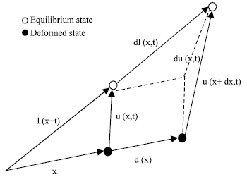 | |
| Fig. 1: | Differential particle displacement in a deformed medium |
However, analysis of anisotropic wave-propagation phenomena, such as shear-wave splitting, could lead to more information, such as strike direction and density of vertical particle within reservoir[11,12] which helps in the understanding of the earth. Transverse isotropy with vertical symmetry axis (TIV) serves as a good introduction to anisotropy for geophysicist and helps to define the basic terminology and methodology for anisotropy studies[1].
Particle displacement and strain field: When the particles of a medium are displaced from their equilibrium positions internal restoring forces arise which lead to oscillatory motion of the medium. Each particle is assigned an equilibrium position vector ![]() and the displacement position vector
and the displacement position vector ![]()
The displacement of the particle located at ![]() in the equilibrium state is defined by Fig. 1.
in the equilibrium state is defined by Fig. 1.
| (1) |
However, since the particle displacement field ![]() is non-zero for rigid motions, it does not itself provide a satisfactory measure of material deformation. A more convenient quantity is:
is non-zero for rigid motions, it does not itself provide a satisfactory measure of material deformation. A more convenient quantity is:
| (2) |
which measures the difference between the distance of two neighboring particles in the equilibrium state and deformed state. In Fig. 1 two displaced particle positions at fixed time are shown for two neighboring particles separated ![]() by in the equilibrium state.
by in the equilibrium state.
The deformation measure ![]() is calculated from
is calculated from ![]() by using relations:
by using relations:
| (3) |
where, ![]() for continuous medium, is the 3x3 matrix made from the derivatives of
for continuous medium, is the 3x3 matrix made from the derivatives of ![]() with respect to
with respect to ![]() . Thus
. Thus
 | (4) |
where, the matrix elements ![]() are termed as components of the strain field.
are termed as components of the strain field.
 | (5) |
The strain field determines the deformation ![]() in terms of the particle displacement
in terms of the particle displacement ![]() and reduces it to zero for all rigid motions.
and reduces it to zero for all rigid motions.
Solids differ widely in their deformabilities. For rigid materials, the displacement gradient must be kept below unity if permanent deformation is to be avoided. For displacement derivatives much smaller than unity, the quadratic terms in equation (5) are negligible and this allows using the linearized strain field:
 | (6) |
Since the strain field is symmetric, one subscript rather than two can specify each component. Following Voigt notation, we can obtain:
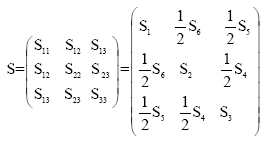 | (7) |
The strain field may also be written as a six-element column matrix rather than a nine-element square matrix, such as follows:
| (8) |
and it can also be decomposed in more simple form by introducing the operator:
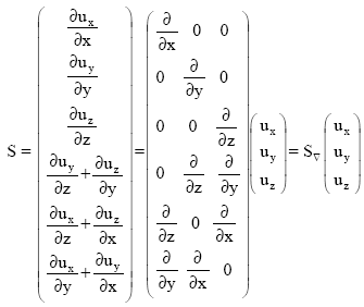 | (9) |
Traction forces and stress field-equation of motion: A method of exciting vibrations in a material body is to apply external forces at its surface. In this case the applied excitation does not act directly on particles within the body but is transmitted to them by means of the Hook forces acting between neighboring particles. To specify these forces, three force components are required for each face of the particle; the traction force acting on the area element facing i direction is vector:
| (10) |
The components ![]() of these forces are called stress components;
of these forces are called stress components; ![]() is the ith component of force acting on the +j face of an infinitesimal volume element at position
is the ith component of force acting on the +j face of an infinitesimal volume element at position ![]() .
.
The abbreviated subscript notation introduced for the strain field can also be used to describe the stress components:
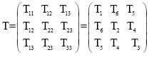 | (11) |
In this case the convention is to omit the factor ½ that appeared in equation (7) and the stress can now be written as a six-element column matrix:
| (12) |
The forces associated with the vibration of material particle are the traction forces applied to its surface by the neighboring particles:
| (13) |
where, ![]() is the normal vector to the surface.
is the normal vector to the surface.
Green’s formula applied on the integrated surface acting on the particle gives:
| (14) |
with ![]() being the divergence of the stress matrix
being the divergence of the stress matrix
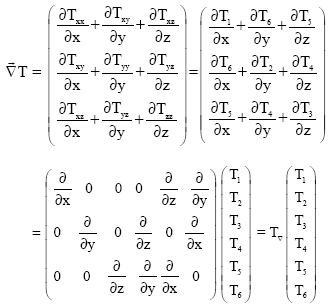 | (15) |
The equation of motion is obtained using Newton’s law:
| (16) |
ρ is the density of the medium and ![]() is the particle velocity.
is the particle velocity.
Hooke’s law: For small deformations it is experimentally observed that the strain in a deformed body is linearly proportional to the applied stress, i.e.
| (17) |
where, c are the elastic stiffness constants.
In the full index notation c is a tensor of order 4 and there are 34 = 81 elastic stiffness constants. These are not all independent, however, since ![]() (because S and T are symmetric matrices), the number of independent constants is reduced to (3+2+1)2 = 36. Some remarks about energy give
(because S and T are symmetric matrices), the number of independent constants is reduced to (3+2+1)2 = 36. Some remarks about energy give ![]() , thus only 6+5+4+3+2+1 = 21 independent constants left. This is the maximum number of elastic constants for any medium. For an isotropic medium, there are only two independent constants
, thus only 6+5+4+3+2+1 = 21 independent constants left. This is the maximum number of elastic constants for any medium. For an isotropic medium, there are only two independent constants ![]() called the Lame’s parameters.
called the Lame’s parameters.
Christoffel equation
By equation (16), we have
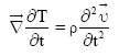 | (18) |
and using equations (15), (17) and (9), the following can be obtained
| (19) |
Equation (19) is a wave equation for general homogeneous media for which a plane wave analysis can be performed. A uniform plane wave ![]() propagating along the direction
propagating along the direction ![]() proportional to
proportional to![]() , where,
, where, ![]() and k is the wavenumber;
and k is the wavenumber; ![]() is the velocity of the advance of wavefront and is called the phase velocity.
is the velocity of the advance of wavefront and is called the phase velocity.
Operators and act on a plane wave like
 | (20) |
After replacing the relevant parts in equation (19) with ![]() and equation (20), the following dispersion relation can be derived
and equation (20), the following dispersion relation can be derived
 | (21) |
where, Γ is a 3x3 matrix called the Christoffel matrix, whose elements are functions only of the plane wave propagation direction ![]() and of the stiffness constants cKL of the medium.
and of the stiffness constants cKL of the medium.
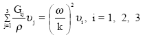
The dispersion relation (21) is an eigenvalues problem (![]() are the eigenvalues). It has the unique solution
are the eigenvalues). It has the unique solution ![]() (i.e. no propagation in the medium!), if the determinant of the system is non-zero; since this is not physically attainable, the determinant should be zero.
(i.e. no propagation in the medium!), if the determinant of the system is non-zero; since this is not physically attainable, the determinant should be zero.
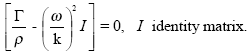 | (22) |
There are 3 possible solutions for the phase velocity ![]() in equation (22), only waves with one of these phase velocities can propagate in the medium.
in equation (22), only waves with one of these phase velocities can propagate in the medium.
Associated with each eigenvalue, there is an eigenvector corresponding to the polarization of the wave propagating with the phase velocity. Mathematically the three eigenvectors are mutually orthogonal, which suggests that physically the three polarizations are in the direction of propagation: one of these is the quasi-longitudinal wave and is simply denoted as P. Another eigenvector is orthogonal to the first one but not to the direction of propagation: this is the quasi-traverse shear wave and is denoted SV. The last eigenvector is orthogonal to the direction of propagation and also to the other eigenvectors: this is the exactly traverse shear wave and is denoted SH.
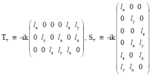
Hexagonal symmetry and vertical axis: Up to now, the hexagonal system has been the anisotropic symmetry most frequently used. This system is of rotational symmetry, which means that the tensor cijkl does not change with rotation around the axis of symmetry. In other words, in the plane perpendicular to this axis, the tensor behaves isotropically. Therefore, the symmetry is also sometimes called transverse isotropy, especially in case when the axis of rotational symmetry coincides with x3----the axis of the coordinate system. With regard to hexagonally symmetric material with a vertical axis of symmetry, matrix ![]() can be expressed as:
can be expressed as:
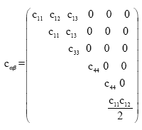 |
The hexagonal symmetry is described by five independent elastic parameters. The coordinate system in which the matrix ![]() is given should be described as
is given should be described as ![]() . In the above case, the axis x3 coincides with the axis of rotational symmetry, while x1, x2 are both located in the isotropic plane.
. In the above case, the axis x3 coincides with the axis of rotational symmetry, while x1, x2 are both located in the isotropic plane.
In the case of the hexagonal symmetry, the Christoffel equation (22) can be expressed as:
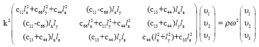 | (23) |
Thus, there are only five independent elastic constants for describing a crystal with hexagonal symmetry: c11, c13, c33, c44, c66.
The propagation vector ![]() could be written as:
could be written as:
| (24) |
where, θ is the angle between the propagation direction and the vertical axis.
Solving the zero-determinant equation (22) yields the solutions  satisfying
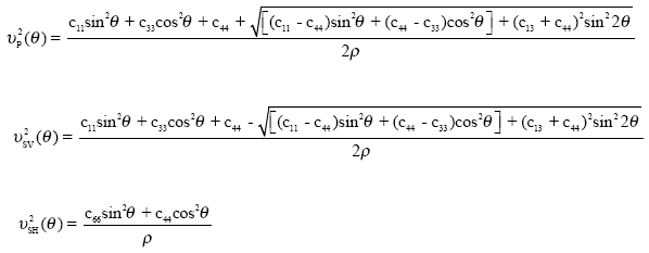 | (25) |
Thomsen’s notations: As introduced by Thomsen[13], it is useful to recast equations (25) using notations involving only two elastic moduli (e.g. vertical P and S velocities) plus three measures of anisotropy. In order to simplify equations (25), these three anisotropy coefficients should be nondimensional and efficient combinations of elastic moduli (c11,…….,c66). Furthermore, they should reduce to zero in case of isotropy. One suitable combinations the author derived is:
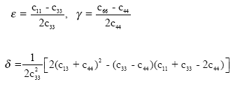 | (26) |
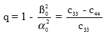
Since the vertical P and S velocities are:
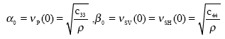 | (27) |
equation (25) can be rewritten as:
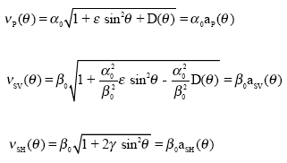 | (28) |
where, D(θ) is given by:
| (29) |
with
 | (30) |
ε, δ and γ are called Thomsen’s parameters and are convenient variables to support calculus.
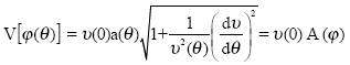
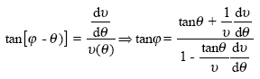
Phase velocity and group velocity: In a general homogeneous elastic medium, where the velocity is constant in any given direction, it is obvious that a particle moves along a straight line; the energy propagates along this line with group velocity, while group angle φ is formed between the direction of propagation and the vertical axis.
However, due to anisotropy, the wavefront is non spherical. The wave vector ![]() is locally perpendicular to the wavefront and the phase angle θ with the vertical axis. The phase velocity that suggests the speed of advance of the wavefront along the direction is given by the Thomsen’s formula (28).
is locally perpendicular to the wavefront and the phase angle θ with the vertical axis. The phase velocity that suggests the speed of advance of the wavefront along the direction is given by the Thomsen’s formula (28).
Figure 2 shows that a point on the wavefront can be reached either by energy traveling with group velocity V(φ) and group angle φ in the direction of energy propagation or by phase traveling with phase velocity V(θ) and phase angle θ in the direction perpendicular to the wavefront. Note that the phase velocity direction does not start from the source point.
Thus, in a homogeneous medium, wavefronts are defined by:
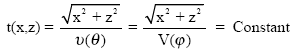 | (31) |
From
 | (32) |
We derive:
| (33) |
which suggests that the traveltime along the ray is a linear function of the source-wavefrontdistance. Also, along a ray of energy propagation, the direction of vector normal to the wavefront is constant ![]() . Thus, θ is irrelevant to time and is constant when φ is fixed.
. Thus, θ is irrelevant to time and is constant when φ is fixed.
The phase velocity is defined as the projection of the group velocity on the vector normal to the wavefront (Fig. 2). Thus, the group velocity is given in terms of the phase velocity as:
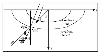 | |
| Fig. 2: | Phase (wavefront) angle θ at two consecutive times and group (ray) angle φ |
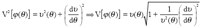 | (34) |
and with the general form of equation (28) we have
 | (35) |
The general relation between group angle φ and phase angle θ is (Fig. 2).
 | (36) |
In anisotropic media, wavefronts traveling outward from a point source are not, in general, spherical as a result of dependence of velocity upon direction of propagation. Shown in Fig. 2 are two wave fronts in space separated by unit time. The group velocity, V(φ), denotes the velocity with which energy travels from the source, while the phase velocity, v(φ), is the velocity with which a wavefront propagates at a local point. Here, the group angle φ specifies the direction of the ray from the source point to the point of interest, while the phase angleφ (also called wavefront-normal angle) specifies the direction of the vector that is normal to the wavefront. In general, they are different at any point of propagation, except at certain singular points.
CONCLUSIONS
This study has presented anisotropy in detail. In particular, Transverse isotropy (TIV) is described by five elastic parameters. This has been achieved by using simplifications of notations introduced by Thomsen, 1986. Furthermore, the group velocity is derived as a function of the group angle from the phase velocity that varies with the phase angle.
REFERENCES
- Crampin, S., 1981. A review of wave motion in anisotropic and cracked Elastic-media. Wave Motion, 3: 343-391.
CrossRefDirect Link