
Yuri Goegebeur
Not Available
Viviane Planchon
Not Available
Jan Beirlant
Not Available
Robert Oger
Not Available
Journal of Applied Sciences
Year: 2005 | Volume: 5 | Issue: 6 | Page No.: 1092-1102


ABSTRACT
The calcium (Ca) content distribution of soil samples collected in several districts of Belgium (Condroz region) is right skewed and long-tailed resulting in frequent large Ca measurements. Robust statistical procedures based on the normal distribution are inappropriate for this kind of data since these will identify a too large number of data as suspicious. Therefore, heavy tailed or Pareto-type distributions are used to model the Ca content in soil samples taking into account the possible relationship with covariates such as pH. For some districts, the largest Ca observations can even be considered as outliers with respect to the conditional Pareto-type model (given a particular pH level). An automatic procedure is proposed to identify such suspicious Ca measurements. In a preliminary step, the generalized Pareto distribution is fitted locally in order to get an idea about the dependence of the tail of the Ca distribution on the covariate pH. Next, the Burr distribution is extended to a regression model by taking its shape parameter as a function of the covariate pH, using the information obtained in the exploratory nonparametric analysis. Suspicious Ca measurements are now identified automatically on the basis of the Burr conditional quantile function.
PDF Abstract XML References Citation
How to cite this article
Yuri Goegebeur, Viviane Planchon, Jan Beirlant and Robert Oger, 2005. Quality Assessment of Pedochemical Data Using Extreme Value Methodology. Journal of Applied Sciences, 5: 1092-1102.
DOI: 10.3923/jas.2005.1092.1102
URL: https://scialert.net/abstract/?doi=jas.2005.1092.1102
DOI: 10.3923/jas.2005.1092.1102
URL: https://scialert.net/abstract/?doi=jas.2005.1092.1102
INTRODUCTION
In agriculture, soil analysis is the best fertilizer and amendment recommendations in the context of managing sail fertility and crop performance. Fertilizers are used to meet crop demand for nutrients while amendments (as lime) are necessary to stabilize and improve both soil structure and water in infiltration and to optimize pH levels.
Recently, a new concept of crop management, called precision farming, has emerged. It permits within-field variation of crop techniques, for instance to adjust fertilizer inputs on the basis of soil sampling and soil analysis. As the development of these techniques increased the demand for soil data, laboratories are now burdened with large data sets. Inevitably, huge data numbers cause concerns about outliners and the quality of the information. Outliner detection methods are therefore essential in the database management, especially before integration of new data sets, in order to provide high quality data to laboratories or extension services.
In this context, the Belgian non-profit organisation REQUASUD (Réseau Qualité Sud i.e. South Quality Network) was created in 1989 to put an analysis service and efficient advices at the practitioner's disposal. REQUASUD developed a centralized soil database which contains more than 150,000 soil chemical composition (pH, KCl, K, Mg, Ca, etc.) records. It also has information about sample origin (zip code), soil texture, soil occupation, previous and recent cultures. The Unit of Geopedology (Gembloux Agricultural University-Belgium) is the reference laboratory for soil analysis and the database is centralized at the Unit of Biometry, Data Management and Agrometeorology (Walloon Agricultural Research center). Detailed studies of the data allow extension services to study physical and chemical properties of agricultural soils and to manage them according to their fertility potential and their ability to support cultures.
The present research is limited to pHKCl and Ca; methods of soil sample extraction are presented in Laroche and Oger[1].
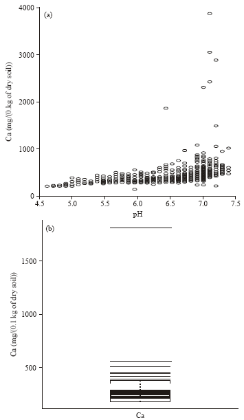 | |
| Fig. 1: | (a) Scatterplot of Ca against pH for one of the districts in the Condroz database, (b) boxplot of Ca measurements at pH = 6.5 |
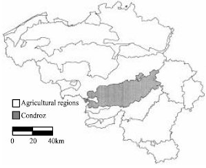 | |
| Fig. 2: | Map of the agricultural regions of Belgium with the localization of the Condroz (grey shaded) |
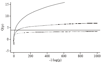 | |
| Fig. 3: | GEV quantile function for γ = 0.25 (solid line),γ= 0 (broken line) and γ= -0.25 (broken dotted line) |
pH, KCL is the result of a pH measurement in a soil salt extract (KCl 0.1 N-quotient soil/solution = 2/5). This determination represents the exchange acidity content and is more stable over time as it is linked to permanent soil characteristics. Ca-content corresponds to the exchangeable Ca-content, i.e., the Ca available for plant nutrition. This part of Ca is formed by compounds that are present in soil solution and that are absorbed on soil colloids. Ca extraction is performed using ammonium acetate 0.5 M with a chelatant EDTA (etylene diamine tetra-acetic acid) 0.02 M and pH fixed to 4.65. Ca-content is measured using a flame atomic absorption and expressed in mg(0.1 kg)-1 of dry soil. The dataset contains nearly 19,000 observations with a mixture of samples coming from crop and meadow soils. Soil samples are extracted from the top horizon (0.20-0.25 meter depth).
Before any analysis or extraction of information from the soil database, identification of suspicious data is needed. For the compound Ca, the distribution conditional on factors such as pH is right skewed and long tailed resulting in frequent large Ca measurements, see for instance the Ca against pH scatterplot given in Fig. 1(a). As a consequence robust statistical procedures based on the normal distribution are not appropriate for this kind of data since these will identify too many large observations as outlying. Figure 1(b) shows the boxplot of the Ca measurements at pH = 6.5. Using the simple rule of thumb (based on the classical Gaussian model) observations that are more than 1.5 times the interquartile range away from the box are suspect, results in 7 observations that deserve further investigation. Extreme value theory offers the appropriate framework for analysing such long tailed data in a more efficient way. However even relative to a heavy tailed model, some really outlying observations occur and need to be identified for further investigations. Analysis based on a heavy tailed model identified as only the largest Ca measurement at pH = 6.5 as suspicious. Extreme value theory has been applied on a part of the database, limited to the Condroz region (Fig. 2). The ultimate aim of the analysis is the development of an automatic procedure to highlight suspicious observations during the process of incorporation of new data into the database in order to guarantee quality.
EXTREME VALUE STATISTICS
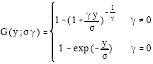
Univariate extreme value theory: Extreme value statistics focuses on characteristics related to the tail of distribution functions such as indices describing tail decay, extreme quantiles, small tail probabilities and (in multivariate settings) indicators of extremal dependence. The tail behaviour of a distribution function is governed by a parameter γ, called the tail index or extreme value index, where tails become heavier as γ increases. This parameter γ is the shape parameter of the Generalized Extreme Value distribution (GEV), with distribution function given by
 | (1) |
μ ε IR is a location parameter and σ>0 is a scale parameter. The use of the GEV in the context of statistics of maxima is motivated by the fact that the distribution of maxima of large samples approximately follows a GEV distribution: if a limiting distribution exists for the largest value in a sample, then it has to be of the form (1). More formally, consider Y1, Y2,....., Yn independent and identically distributed (i.d.) random variables with common distribution function FY and denote the associated sequence of ascending order statistics by Y1, n≤Y2, n≤...≤Yn,n. Then for a very broad class of distribution functions
| (2) |
provided the sample size n is sufficiently large. A formal mathematical derivation of the above result was given in Fisher and Tippett[2] and Gnedenko[3]. Note that the role of the GEV as limiting distribution of sample maxima is in some sense akin to the role the normal distribution plays for sample means.
Figure 3 illustrate the importance of the extreme value index γ as shape parameter of the GEV. Let Q denote the quantile function associated with distribution function F. Figure 3 shows the GEV quantile function given by:
as a function of -1/log p for some values of γ; here we set μ = 0 and σ = 1. Inspecting the 99th percentile, Q(0.99), (corresponding to the horizontal value 1 = log(0.99) = 99.4992) it is clearly observe an increase in quantile level with increasing γ. Note that for γ = -0.25 (broken-dotted line) the GEV has a finite right endpoint (namely 4) represented by the horizontal reference line, while for the cases γ = 0 (broken line) and γ = 0.25 (solid line) extrapolation will lead to an infinite limit.
This study concentrates on heavy tailed or Pareto-type distributions i.e. distributions for which there exists a γ>0 such that for a sufficiently high threshold u, the conditional distribution of the relative excesses Y/u given Y>u, denoted FY/μ |Y>u, approximately follows a strict Pareto distribution, or more formally
| (3) |
It was shown[3] that in case γ>0, conditions (2) and (3) are equivalent. Popular models of this class are, next to the strict Pareto distribution (for which (3) holds with equality for all u), the Burr, the generalized Pareto, the loggamma, the t and the F distributions.
Applications of model (3) can be found in scientific disciplines such as finance, insurance, reliability theory, environmetrics, geology and climatology. Here (3) will be used to model the Ca-content in soil samples taken in several districts in the Condroz, hereby taking into account the possible influence of independent variables or covariates.
The fit of a statistical model to a random sample Y1, Y2,....., Yn can be visually assessed by inspection of a quantile-quantile or QQ plot. Indeed, in case of a good fit by the proposed reference distribution, the ordered data which serve as empirical quantiles are expected to be in line with their expected values under the fitted model. Since log-transformed Pareto distributed data are exponentially distributed, it is natural to consider an exponential quantile plot based on the log-transformed data, leading to a Pareto quantile plot, i.e.
In case the data originate from a strict Pareto distribution, the Pareto quantile plot will show a straight line pattern of which the slope is given by the extreme value index γ. Indeed, for the strict Pareto distribution log Q(1-p) = -γ log p, 0 < p < 1. For Pareto-type distributions this linearity can only be observed for the largest observations:
Again the slope of the linear part will approximate γ.
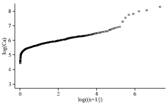 | |
| Fig. 4: | Pareto quantile plot of the variable Ca for one of the districts in the Condroz database |
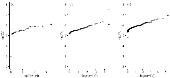 | |
| Fig. 5: | Pareto quantile plots of the Ca measurements at (a) pH = 6, (b) pH = 6.5 and (c) pH = 7 |
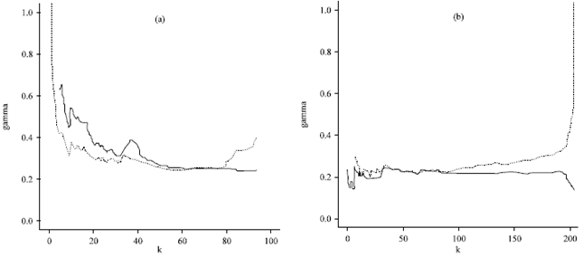 | |
| Fig. 6: | Hk,n (broken line) and (solid line) of the Ca measurements as a function of k at (a) pH = 6.5 and (b) pH = 7 |
Except for the last 7 points, the Pareto quantile plot is linear in the larger observations. The very largest observations that do not follow the ultimate linearity of the Pareto quantile plot can be considered as outliers with respect to the Pareto-type model. However, in this analysis is was conditioned on the city but did not take into account the possible link with other covariates such as pH level. However, as can be seen from the Ca versus pH scatter plot given in Fig. 1a both variables seem to be positively associated. Moreover, extreme Ca measurements tend to occur more often at the higher pH levels, indicating the need for a tail analysis conditional on the covariate pH.
When covariate information is available, the appropriateness of model (3) for the conditional distribution of the dependent variable given the covariates can be visually assessed by inspection of Pareto quantile plots of the response observations within narrow bins in the covariate space. This is illustrated in Fig. 4 where the Pareto quantile plots are given for the Ca measurements conditional on (a) pH = 6, (b) pH = 6.5 and (c) pH = 7. Clearly all quantile plots are approximately linear in the extreme values indicating a good fit of the Pareto-type model to the conditional distribution of the variable Ca given a pH level. The largest Ca measurement in Fig. 5b does not follow the straight line pattern set by the other large observations; hence this observation can be considered as an outlier with respect to the conditional Pareto-type distribution and should receive special attention. These observations form the basis for the automatic procedure for highlighting such suspicious observations.
Quantile based estimation of γ: The extreme value literature on the estimation of the extreme value index γ using a sample of i.i.d. random variables is very elaborate. Hill[4] introduced the following popular estimator for γ.
| (4) |
The Hill estimator measures the average increase of the Pareto quantile plot above an anchor point ![]() and hence can be interpreted as a slope estimator. Several other authors have recognized and exploited the potential of QQ plots in estimating γ > 0. We refer to Beirlant et al.[5], Kratz and Resnick[6] and Schultze and Steinebach[7]. Other well know alternative tail index estimators are the kernel estimators[8] and the moment estimator[9]. Remark that this estimator is to be computed for k = 1,..., n-1. The resulting estimates are often plotted against k (or log k). Making an appropriate choice of k is not always easy due to the large variability of the values Hk,n over k. To this end, Beirlant et al.[10] derived the following approximate representation for log-spacings of successive order data
and hence can be interpreted as a slope estimator. Several other authors have recognized and exploited the potential of QQ plots in estimating γ > 0. We refer to Beirlant et al.[5], Kratz and Resnick[6] and Schultze and Steinebach[7]. Other well know alternative tail index estimators are the kernel estimators[8] and the moment estimator[9]. Remark that this estimator is to be computed for k = 1,..., n-1. The resulting estimates are often plotted against k (or log k). Making an appropriate choice of k is not always easy due to the large variability of the values Hk,n over k. To this end, Beirlant et al.[10] derived the following approximate representation for log-spacings of successive order data
| (5) |
with bn,k ε IR, ρ < 0 and Fj, j = 1,2,..., k, independent standard exponential random variables, from which γ can be estimated jointly with bn,k and ρ using the maximum likelihood method. Compared to the Hill estimator, the maximum likelihood estimator for γ. based on (5) is typically stable over k and performs better with respect to bias. Figure 6 shows the Hill (broken line) and the maximum likelihood estimates (solid line) for the tail index of the conditional distribution of Ca given (a) pH = 6.5 and (b) pH = 7 as a function of k. Note the influence of the outlying Ca measurement at pH = 6.5 on the γ estimates, especially for the smaller k-values.
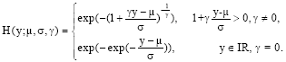
POT estimation of γ: Next to the above described quantile based estimation procedures, the real valued index γ can also be estimated using the limit theorems that form the basis of extreme value theory. A first possibility is the method of block maxima where the GEV given in (1) is fitted to a sample of maxima[11]. This classical approach received considerable criticism, mainly because of its inefficient use of the available data. Indeed, next to the maximum, other large order statistics contain information about the tail of the distribution and hence can be used to estimate γ. This is the basic idea behind the so-called Peaks Over Threshold (POT) approach where the Generalized Pareto Distribution (GPD), given by
 | (6) |
with σ > 0 and support y > 0 if γ≥0 and 0 < y < σ/|γ| if γ < 0, is fitted to the exceedances over a sufficiently high threshold. This approach can be motivated as follows. Let u denote a threshold value and consider Fu the conditional distribution of the absolute excesses Y-u given Fγ>u. Pickands[12] showed that for FY satisfying (2)
for some σ(u)>0, provided the threshold u is set sufficiently high. The practical implication of this result is that for a sufficiently high threshold μ the conditional distribution of exceedances can be well approximated by the GPD. The parameters of the GPD can be estimated with the maximum likelihood method[13,14], the method of (probability-weighted) moments[15] or the elemental percentile method[16].
REGRESSION ANALYSIS
Parametric regression analysis based on extreme thresholds: A straightforward way to include covariate information is to consider one or more of the parameters of (1), (3) or (6) as a function of the covariates. For instance, model (3) can be extended by modelling γ as a function of the covariate x
| (7) |
Next, these extended models are fitted to respectively sample maxima or exceedances over a sufficiently high threshold. The function γ(x) yields information about the tail heaviness of the conditional distribution of the dependent variable Y given the covariate x. Such an approach requires knowledge of the functional form to use for the parameter functions. When working with the GPD one is faced with the additional issue that the threshold should depend on the covariates in order to take the relative extremity of the observations into account[17-19].
Nonparametric regression estimation of γ: Here the nonparametric approach will be based on local maximum likelihood fits of the GPD, discussed in Beirlant and Goegebeur[20], as an exploratory tool to get an idea about the functional form to use for γ in a subsequent completely parametric analysis based on a specific Pareto-type model, i.e. assuming a particular functional form to describe the deviation from the strict Pareto distribution. This procedure also takes care of the issue of a covariate dependent threshold.
Consider a sample (Y1, x1,),....,(Yn, xn,) of independent observations from (7), so it is assumed the conditional distribution of the dependent variable Y given the covariate x is of Pareto-type or heavy tailed and assume interest is in estimating γ at x*. Following the GPD approach discussed above we fix a threshold (note that the threshold depends on x*; for more details about achieving this dependence in practice we refer to Beirlant and Goegebeur[20] and denote by ![]() the exceedances over
the exceedances over ![]() with j the index in the original sample of the i-th exceedance. Re-index the covariate observations associated with the exceedances accordingly. Pickands’ result states that for a sufficiently high , the conditional distribution of
with j the index in the original sample of the i-th exceedance. Re-index the covariate observations associated with the exceedances accordingly. Pickands’ result states that for a sufficiently high , the conditional distribution of ![]() can be well approximated by the GPD. Note that, since we are dealing with the regression case, the parameters γ and σ may depend on x*. The unknown values γ(x*) and σ(x*) are estimated nonparametrically by local fitting of the GPD to the exceedances Zi,x*, i = 1,..., Nx*, hereby replacing the true parameter functions by their respective polynomial approximations obtained from a Taylor series expansion around x*:
can be well approximated by the GPD. Note that, since we are dealing with the regression case, the parameters γ and σ may depend on x*. The unknown values γ(x*) and σ(x*) are estimated nonparametrically by local fitting of the GPD to the exceedances Zi,x*, i = 1,..., Nx*, hereby replacing the true parameter functions by their respective polynomial approximations obtained from a Taylor series expansion around x*:
and
where, ![]() Clearly σ(x*) = β10 and γ(x*) = β20 . Together with local fitting of the GPD one also involves a weight or kernel function K, defined on [-1,1] and a bandwidth parameter h which rescales K as
Clearly σ(x*) = β10 and γ(x*) = β20 . Together with local fitting of the GPD one also involves a weight or kernel function K, defined on [-1,1] and a bandwidth parameter h which rescales K as ![]() and which determines the amount of smoothing. Enlarging h, more data around x* are incorporated and the variance will decrease; but if h is too large bias can be introduced since distant observations not necessarily give the correct story on the behaviour at x*. The local polynomial maximum likelihood estimator
and which determines the amount of smoothing. Enlarging h, more data around x* are incorporated and the variance will decrease; but if h is too large bias can be introduced since distant observations not necessarily give the correct story on the behaviour at x*. The local polynomial maximum likelihood estimator ![]() maximizes
maximizes
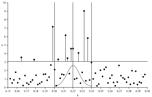 | |
| Fig. 7: | Graphical illustration of the nonparametric estimation procedure |
 | |
| Fig. 8: | (a) Local polynomial maximum likelihood estimates of γ using p = 1, h = 0:5 and k = 40 (solid line), k = 50 (broken line), k = 60 (broken-dotted line) as a function of pH and (b) local polynomial maximimum likelihood estimates of γ using p = 1, h = 0:5, k = 40 (solid line) and best fitting exponential link function (broken line) |
 | |
| Fig. 9: | Some Burr density functions (β = 1 and some values for τ and λ) |
 |
with respect to (β1, β2), where g denotes the GPD density function given by
| (8) |
This yields estimates for σ and γ and their derivatives up to order p1, respectively p2. Beirlant and Goegebeur[20] proved consistency and asymptotic normality of this estimator. Figure 6 illustrates the estimation of γ at x* = 0.22 using = 3 and h = 0.02. The exceedances are given by the vertical line segments. The threshold is exceeded by 11 observations but only the exceedances with x component in the interval [0.20,0.24] will be used in the estimation.
The maximum likelihood estimation of the GPD to the 8 exceedances involves replacing σ(xi) and γ(xi) by their polynomial approximation obtained from a Taylor series expansion and the weighting of contributions to the log-likelihood function by a kernel function (in the graphical illustration we plotted a normal kernel function). Maximizing this kernel-weighted log-likelihood function yields the desired parameter estimates.
In Fig. 8a the results of the local maximum likelihood estimation applied to the Condroz data are given. This figure shows the nonparametric estimates for γ obtained with and h = 0.5 as a function of pH and this for different values of k. Here k denotes the number of exceedances used in the local estimation, i.e. the threshold is set at the (k+1)-th largest response observation within the interval [x*-h, x*+h]. This exploratory plot clearly indicates that an exponential link function may be a good choice to model γ in terms of pH. This is further illustrated in Fig. 8b, where we compare the nonparametric γ estimate for (x), p1 = p2 = 1, h = 0.5 and k = 40 with the -in a least squares sense-best fitting exponential function.
PEDOCHEMICAL RESULTS-BURR MODELLING
The extreme value methodology based on the semi-parametric Pareto-type model discussed so far focuses mainly on tail modelling. However, we clearly recognise the need for completely parametric models that are capable to fit well both the tail and the more central parts of the Ca domain conditional on pH. Moreover, such completely parametric models are easier to incorporate in a fully automatic procedure designed to highlight suspicious Ca measurements.
One flexible class of parametric models is given by the Burr(β, τ, λ) distribution, with distribution function
| (9) |
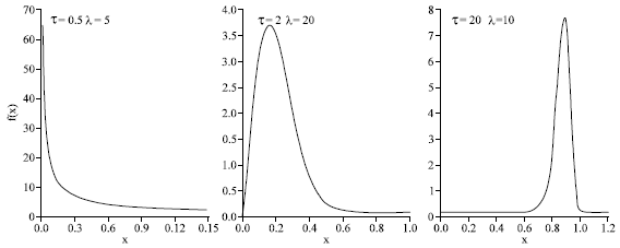
Note that this distribution is of Pareto-type with γ = 1/λτ. The Burr(β, τ, λ) density function fY(y) = λβλτyτ-1/(β+yτ)λ+1 is unimodal, with mode at (β(τ-1)/(λτ+1)1/τ, if τ>1 and L-shaped for τ≤1, so the parameter τ is a shape parameter. On the other hand, the scale of the Burr distribution is determined by the parameter β1/τ. Figure 9 show Burr densities with β = 1 and various values for λ and τ. Rodriguez[21] compared several distributions and studied their flexibility using a moment-ratio diagram. The area covered by the Burr(β, τ, λ) distribution contains popular models such as the normal, the logistic and the Weibull distributions.
When including covariate information in a statistical analysis, the conditional distribution of the response variable Y given the covariate x is considered. Allowing one or more of the parameters to vary with x, the Burr(β, τ, λ) distribution given by (9) can be extended to a regression model. This study will focus on one of the two model parameterizations introduced in Beirlant et al.[22].
Assuming the shape parameter τ depends on x we have
Y|x~Burr(β, τ (x), λ)(10) | (10) |
Various functional forms can be used for τ(x). Given the results of the nonparametric analysis based on local fits of the GPD and the fact that for the Burr(β, τ, λ) distribution γ = 1/λτ, an exponential link function is a natural choice, so τ(x) = exp(θ0+θ1x). A second parameterization can be derived from the relation between the Burr and the generalized logistic distribution. Indeed, taking a log-transform of the dependent variable together with the parameterization β(x) = exp(τ(θ0+θ1x)) results in a generalized logistic location-scale model
| (11) |
Note that this second parameterization leads to a covariate dependent scale parameter: β1/τ = exp (θ0+θ1x).
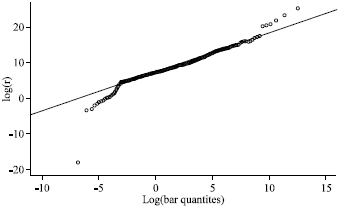 | |
| Fig. 10: | Burr residual quantile plot of r1, ...., rn |
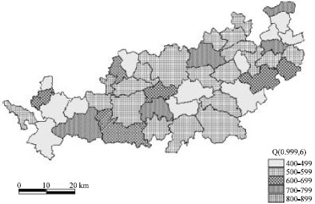 | |
| Fig. 11: | Geographical variation of Q(0.999; 6) in the Condroz region |
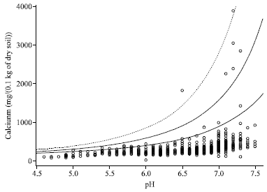 | |
| Fig. 12: | Scatter plot of Ca against pH with Q(p; pH) superimposed: (a) p = 0.99 (solid line), (b) p = 0.999 (broken line) and (c) p = 0.9999 (broken-dotted line) |
Regression models based on this second parameterization do not provide flexibility for accurate tail modelling and hence will not be further considered in this paper.
Beirlant et al.[22] discuss maximum likelihood estimation of the parameters of (10). As already introduced in the previous section, the fit of a statistical model to a dataset can be visually assessed by inspection of QQ plots. Under (10), the transformation
removes the dependence on the covariate values xi:
| (12) |
Further, since Y1,..., Yn are independent, the random variables R1,...., Rn are i.i.d. random variables and can be considered as generalized residuals. These can be used to construct a Burr quantile plot to validate model (12). The quantile function associated with (12) is given by
or equivalently, after taking a log-transform
The fit of model (12) to the data can be evaluated by comparing the log-transformed residuals with the above log-transformed quantile function. The graphical presentation of this evaluation is the Burr quantile plot where points have as coordinates:
 |
Clearly, in case model (12) fits the data well, a straight line pattern will arise. In this case the slope of a straight line fitted to the Burr quantile plot will be approximately 1 while the intercept estimate will approximate log β. Figure 10 shows the Burr residual quantile plot for regression model (10) with Y = Ca-content and x = pH level for the city discussed in the previous section. The correlation coefficient between the ordered log-residuals and the corresponding Burr quantiles approximates 0.97.
We now turn to the detection of suspicious Ca measurements. In this process, the Burr quantile function
| (13) |
plays a crucial role. Indeed, Q(p) gives the level that will be exceeded-on average-once in 1/(1-p) cases. If p is taken large enough, i.e. p>1-1/n, then Ca measurements that exceed Q(p) are clearly suspicious. The conditional quantile function, Q(p; x), can be obtained by taking one or more of the parameters as a function of the covariates. The Fig. 11 gives an idea about the geographical variability of the 0.999 quantiles conditional on pH = 6; here Q(0.999; 6) was recoded using 5 levels. These are obtained by plugging the maximum likelihood estimates obtained under (10) into the Burr quantile function (13). Fig. 11 shows results consistency in the spatial distribution of conditional quantiles for adjoining districts while parameters have been calculated independently for each district. These results may be interpreted by different soil maps. Suspicious Ca measurements can be detected graphically by superimposing the estimated conditional quantile function on the Ca versus pH scatterplot. This is illustrated in Fig. 12 for the Burr regression model (10) using p = 0.99 (solid line), p = 0.999 (broken line) and p = 0.9999 (broken-dotted line).
CONCLUSIONS
During recent years huge amounts of pedochemical data are made available for soil analysis. In the Belgian context, the nonprofit organisation REQUASUD developed a centralized database containing over 150,000 soil records. Of course, before any analysis or extraction of data from such a source one has to assure the quality of data. This study developed an automatic procedure for the identification of suspect Ca measurements, hereby taking into account the possible relation with other factors such as pH level. In an exploratory step, the generalized Pareto distribution was fitted locally to exceedances over a high threshold in order to get an idea about the tail dependence of the Ca distribution on the covariate pH. This information was used as input for a second step where a flexible global parametric model was fitted to all data, not just the tail observations. Suspicious Ca measurements are identified on the basis of the conditional Ca quantile function. This procedure could be easily improved by stratification of the dataset according to soil occupancy (crop, meadow). Further, in the present study the fact that the data from a particular district may represent a mixture of different types of soils has not taken into account. Currently, the REQUASUD database does not contain information about this underlying structure. However, following the widespread use of GPS systems, future research projects will focus on the identification and estimation of mixtures of Pareto-type models in presence of covariates.
ACKNOWLEDGEMENT
The authors take pleasure in thanking Jean Laroche (Gembloux Agricultural University, Unit of Geopedology, Belgium) for providing interesting and useful comments.
REFERENCES
- Hill, B., 1975. A simple general approach to inference about the tail of a distribution. Ann. Stat., 3: 1163-1174.
Direct Link - Hosking, J. and J. Wallis, 1987. Parameter and quantile estimation for the generalized pareto distribution. Technometrics, 29: 339-349.
Direct Link - Castillo, E. and A.S. Hadi, 1997. Fitting the generalized Pareto distribution to data. J. Am. Stat. Assoc., 92: 1609-1620.
Direct Link